Day 2 - Take home exercise

Notes and instructions

Answer script

You are expected to save your answer under R-cafe/day2/takehome.R

Piping

It is expected that the exercise answers will be mainly using the pipe operators %>%, instead of putting functions inside each other

Dataset

Same for day 1 exercise, we will also use covid_cases.rds under R-cafe/day1/data/covid_cases.rds for this exercise.

Exercises

Task 1: Data import

• Read data from R-cafe/day1/data/covid_cases.rds

• Load the tidyverse meta-package into R

suppressPackageStartupMessages(library(tidyverse))

covid_cases <- read_rds("../data/covid_cases.rds")

Note

A “meta-package” is a package that contains other packages. Remember, tidyverse is just a collection of packages.

Task 2: Data cleaning and filtering

• Does the data follow the tidy data standard? (refer to session 2 slides)

  • If not, pivot the data into a tibble that follows the tidy data standard

• Do some quick skim on the data. Do the variable values make sense given its type?

  • If not, filter out incorrect/impossible data

• Filter the data so that we only have week 3-12 of 2020

• Save the results back into covid_cases

covid_cases <- covid_cases %>%
  pivot_longer(
    -date,
    names_to = "country",
    names_pattern = "cases_(.+)",
    values_to = "cases"
  ) %>%
  mutate(week = week(date)) %>%
  filter(cases > -1, week < 3 + 10)

Tip: pivotting

• If your data is not tidy data:

  • “Lengthens” the data using tidyr::pivot_longer(), i.e. less columns, more rows

  • “Widens” the data using tidyr::pivot_wider(), i.e. less rows, more columns

Tip: data skimming and cleaning

• Use skimr::skim() such as in day 1 exercises to quickly look at the data

• The main variable here is case counts from each country. They should have a numeric type and should not be lower than 0. You can’t have negative case counts

• You can remove or filter undesirable values using dplyr::filter()

Task 3: Data transformation

• Using the covid_cases object created in Task 2:

  • Group the data and calculate the total number of cases per country

  • Select the top 5 countries with highest total cases

  • Extract the country codes and save them into a new object, e.g. top_countries

top_n <- 5 # optional
top_countries <- covid_cases %>%
  group_by(country) %>%
  summarise(total_cases = sum(cases)) %>%
  slice_max(total_cases, n = top_n) %>%
  pull(country)

• Use the covid_cases object created in Task 2 again:

  • Group the data again, calculate the total number of cases per country again

  • Modify the country column:

    • So that we only keep the names of countries in the top 5 (generated above). Countries on in the top 5 will be changed to "Others"

    • Turn this column into a factor type (refer to session 1 slides using the forcats package (already in tidyverse)

    • Group the data again, this time, group by date and country

    • Calculate the total number of cases per date per country

    • Create a new column called pct_cases, which is the percentage of total cases per date per country

    • (Optional) remove rows with NA from the tibble

    • There are many ways to do this part of the task

  • Save all of this into a new object, e.g. plot_data

plot_data <- covid_cases %>%
  group_by(country) %>%
  mutate(total_cases = sum(cases)) %>%
  ungroup() %>%
  mutate(
    country = fct_lump_n(country, n = top_n, w = total_cases, other_level = "Others") %>%
      fct_relevel("Others", after = Inf)
  ) %>%
  group_by(date, country) %>%
  summarise(total_cases = sum(cases)) %>%
  mutate(
    pct_cases = total_cases / sum(total_cases) * 100
  ) %>%
  drop_na() %>%
  suppressMessages()

Tip: data grouping and summarisation

• Group data into groups with dplyr::group_by() and ungroup data with dplyr::ungroup()

• Summarise each group into a single row with dplyr::summarise()

• You can have multiple groups at the same time. For example:

covid_cases %>%
  group_by(date, country) %>%
  summarise(total_cases = sum(cases))

`summarise()` has grouped output by 'date'. You can override using the
`.groups` argument.

• You can choose not to summarise, but add a new column to each group with dplyr::mutate(). For example:

covid_cases %>%
  group_by(country) %>%
  mutate(total_cases = sum(cases))

This will create a new column total_cases that contains the sum of cases for each country without reducing each group into a single row like summarise(). Values will be duplicated for each group.

Tip: get top n values in a tibble

• You can select rows with the top n values in a tibble using dplyr::slice_max()

Tip: get values of a column in a tibble

• You can extract values from a columns in a tibble using dplyr::pull()

Tip: turn a tibble column into a factor

• You can create and work with factors inside a tibble using the forcats package (already in tidyverse)
• You can “lump”, or gather, factor levels that are not frequent with forcats::fct_lump_n()

Task 4: Data visualization

• Using ggplot2, try your best to generate the following figure:

plot_data %>%
  ggplot(aes(x = date, y = pct_cases, fill = country)) +
  geom_area() +
  scale_y_continuous(
    "Percent of total cases",
    breaks = seq(0, 100, 10),
    labels = paste0(seq(0, 100, 10), "%")
  ) +
  scale_x_date(
    "Date",
    date_breaks = "1 week", date_labels = "W%W",
    minor_breaks = NULL
  ) +
  scale_fill_discrete(
    "Country",
    labels = c(
      "chn" = "China",
      "deu" = "Germany",
      "esp" = "Spain",
      "ita" = "Italy",
      "usa" = "USA"
    )
  ) +
  ggtitle("Percentage of COVID case counts per country for the first 10 weeks of 2020")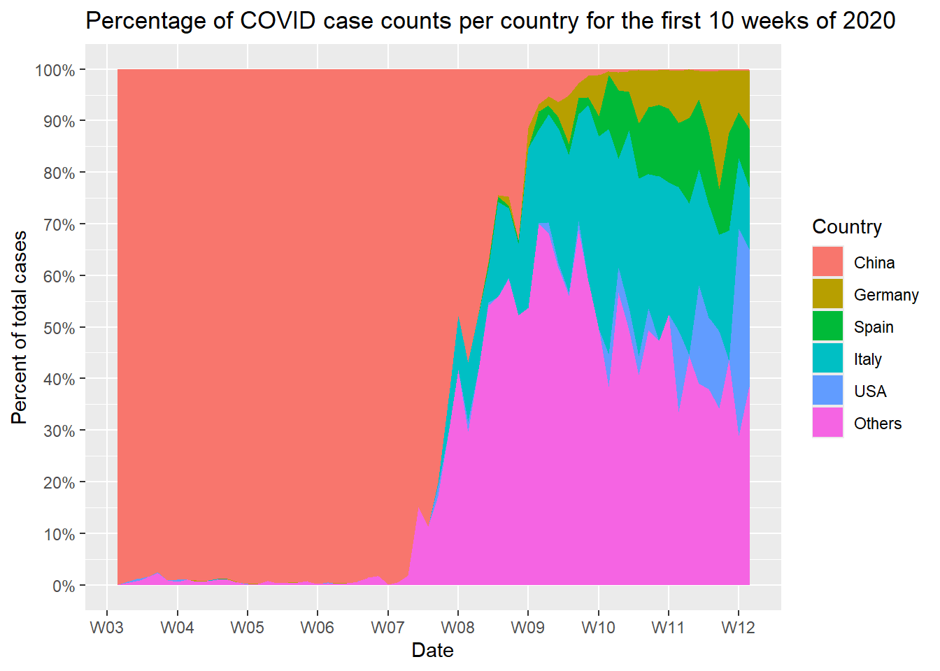

Tip: how do I draw that??

• ggplot2 reference page is very useful
• Here are all the functions used to generate the plot above, in sequence:
  • ggplot()
  • geom_area()
  • scale_y_continuous()
  • scale_x_date()
  • scale_fill_discrete()
  • ggtitle()
  • Every function is connected with the + operator