Equity in Vaccine Access in Ho Chi Minh City

1 Measles vaccine coverage

Code

library(tidyverse)
library(lubridate)
library(janitor)
library(stringi)
library(patchwork)
library(vegan)
invisible(Sys.setlocale("LC_TIME", "English"))
df_raw <- readRDS("D:/OUCRU/assigned github/vac_coverage/data/vaxreg_hcmc_measles.rds")

Code

## data cleaning
df <- df_raw %>% na.omit() %>% 
                 subset(date_m1 > dob & 
                        date_m2 > dob & 
                        date_m1 < date_m2 &
                        year(date_m2) <= 2024 &
                        year(date_m1) >= min(year(df_raw$dob))) 

Vaccine shortage public started in May 2022 source

2 Vaccine coverage (1st and 2nd dose) in Ho Chi Minh city

Code

## vaccine coverage 1st and 2nd dose
date_compute <- seq(as.Date("2022-09-01"),as.Date("2024-11-20"),by = "weeks")

## second dose
out_fn <- data.frame()

for (i in 1:length(date_compute)){
  cov <- df %>% 
    mutate(
      age = decimal_date(date_compute[i]) - decimal_date(dob),
      is_m2 = if_else(date_m2 <= date_compute[i], 1, 0))  %>% 
    filter(age >= 1, age <= 5) %>% 
    summarise(m2 = sum(is_m2, na.rm = T), n = n(), cov = m2/n)
  
  cov_2w <- df %>% 
    mutate(
      age = decimal_date(date_compute[i]) - decimal_date(dob),
      is_m2 = if_else(date_m2 <= date_compute[i] %m-% weeks(2), 1, 0))  %>% 
    filter(age >= 1 + 0.5/12, age <= 5 + 0.5/12) %>% 
    summarise(m2 = sum(is_m2, na.rm = T), n = n(), cov = m2/n)
  
  out <- data.frame(date = as.Date(date_compute[i]),
                    cov = as.numeric(cov$cov),
                    cov_2w = as.numeric(cov_2w$cov))
  
  out_fn <- rbind(out_fn,out)
}


## first dose
out_fn1 <- data.frame()

for (i in 1:length(date_compute)){
  
  cova <- df %>% 
    mutate(
      age = decimal_date(date_compute[i]) - decimal_date(dob),
      is_m1 = if_else(date_m1 <= date_compute[i], 1, 0))  %>% 
    filter(age >= 0.75, age <= 5) %>% 
    summarise(m1 = sum(is_m1, na.rm = T), n = n(), cov = m1/n)
  
  cov_2wa <- df %>% 
    mutate(
      age = decimal_date(date_compute[i]) - decimal_date(dob),
      is_m1 = if_else(date_m1 <= date_compute[i] %m-% weeks(2), 1, 0))  %>% 
    filter(age >= 0.75 + 0.5/12, age <= 5 + 0.5/12) %>% 
    summarise(m1 = sum(is_m1, na.rm = T), n = n(), cov = m1/n)
  
  outa <- data.frame(date = as.Date(date_compute[i]),
                     cov = as.numeric(cova$cov),
                     cov_2w = as.numeric(cov_2wa$cov))
  
  out_fn1 <- rbind(out_fn1,outa)
}


## plot

vac_co <- ggplot()+
  geom_line(data = out_fn,aes(x = date,y = cov*100,color="2"))+
  geom_line(data = out_fn1,aes(x = date,y = cov*100,color="1"))+
  scale_y_continuous(limits = c(0, 100), breaks = seq(0,100,by = 10)) +
  labs(x = "Date",y = "Vaccine coverage (%)")+
  scale_x_date(breaks = "4 month",
               date_labels= "%b %Y",
               limits = c(as.Date("2022-09-01"),as.Date("2024-11-20")))+
  theme(axis.text.x = element_text(angle = 45,size = 8,
                                   hjust=1))+
  scale_color_manual(name="Dose", values=c("1"="red", "2"="blue"))+
  theme_bw()

vac_co2w <-ggplot()+
  geom_line(data = out_fn,aes(x = date,y = cov_2w*100,color="2"))+
  geom_line(data = out_fn1,aes(x = date,y = cov_2w*100,color="1"))+
  scale_y_continuous(limits = c(0, 100), breaks = seq(0,100,by = 10)) +
  labs(x = "Date",y = "Vaccine coverage with 2-week hypothesis (%)")+
  scale_x_date(breaks = "4 month",
               date_labels= "%b %Y",
               limits = c(as.Date("2022-09-01"),as.Date("2024-11-20")))+
  theme(axis.text.x = element_text(angle = 45,size = 8,
                                   hjust=1))+
  scale_color_manual(name="Dose", values=c("1"="red", "2"="blue"))+
  theme_bw()

Code

vac_co | vac_co2w

3 Coverage

Code

district <- unique(df$district)

out_d <- data.frame()
out_d1 <- data.frame()

for (k in 1:length(district)){
  dfd <- df %>% filter(district == district[k])
  for (i in 1:length(date_compute)){
    cov <- dfd %>% 
      mutate(
        age = decimal_date(date_compute[i]) - decimal_date(dob),
        is_m2 = if_else(date_m2 <= date_compute[i], 1, 0))  %>% 
      filter(age >= 1, age <= 5) %>% 
      summarise(m2 = sum(is_m2, na.rm = T), n = n(), cov = m2/n)
    
    cov_2w <- dfd %>% 
      mutate(
        age = decimal_date(date_compute[i]) - decimal_date(dob),
        is_m2 = if_else(date_m2 <= date_compute[i] %m-% weeks(2), 1, 0))  %>% 
      filter(age >= 1 + 0.5/12, age <= 5 + 0.5/12) %>% 
      summarise(m2 = sum(is_m2, na.rm = T), n = n(), cov = m2/n)
    
    out_d1 <- data.frame(district = as.character(district[k]),
                         date = as.Date(date_compute[i]),
                         cov = as.numeric(cov$cov),
                         cov_2w = as.numeric(cov_2w$cov))
    
    out_d <- rbind(out_d,out_d1)
  }  
}

meancv <- out_d %>% 
  group_by(district) %>% 
  summarise(mean = mean(cov)) 

sorted <- meancv[order(-meancv$mean),]

vac_cov <- out_d %>% mutate(dis = factor(district,
                              levels = as.character(sorted$district))) %>% 
ggplot()+
  geom_line(aes(x = date,y = cov*100,color="2"))+
  scale_y_continuous(limits = c(0, 100), breaks = seq(0,100,by = 10)) +
  labs(x = "Date",y = "Vaccine coverage (%)")+
  scale_x_date(breaks = "4 months",
               date_labels= "%b %Y",
               limits = c(as.Date("2022-09-01"),as.Date("2024-11-20")))+
  facet_wrap(vars(dis),ncol = 1)+
  scale_color_manual(name="Dose", values=c("1"="red", "2"="blue"))+
  theme_bw()+
  theme(axis.text.x = element_text(angle = 45,size = 8,hjust=1),
        axis.text.y = element_text(size = 6))

4 Timely vaccination

Code

week <- seq(as.Date("2022-05-01"),as.Date("2024-07-01"),by = "month")

dttlv <- df[,c("dob","district","date_m1","date_m2")] 
out_timely <- data.frame()

for (k in 1:length(district)){
  td <- subset(dttlv, district == district[k]) 
  for (i in 1:length(week)){
    td$lackd <- week[i]
    td$ageuntil <- decimal_date(td$lackd) - decimal_date(td$dob)
    
    ## subset children aged from 9 months to 9 months 2 weeks at chosen time
    slec <- td[td$ageuntil >= 0.75 & td$ageuntil <= 0.75 + 0.5*(1/12),]
    
    slec$agevac <- decimal_date(slec$date_m1) - decimal_date(slec$dob)
    slec$vac_on_date1 <- ifelse(slec$agevac < slec$ageuntil + 1/12,1,0)
    slec$vac_on_date1 <- replace(slec$vac_on_date, is.na(slec$vac_on_date1),0)
    
    re <- slec %>% group_by(vac_on_date1) %>% count()  
    
    if(nrow(re) == 1){
      re[2,] <- re[1,]
      re[1,1] <- 0  
      re[1,2] <- 0  
    } 
    
    cus <- data.frame(district = district[k],
                      date = week[i],
                      per = as.numeric(re[2,2])/(as.numeric(re[2,2])+as.numeric(re[1,2])))
    out_timely <- rbind(out_timely,cus)
  }
}

5 IPSUM analysis

Code

ipsum <- read_csv("data/GEO1_VN2019_79.csv")

ipsum$district <- case_when(
  ipsum$GEO2_VN == 704079760 ~ "Quận 1",
  ipsum$GEO2_VN == 704079761 ~ "Quận 12",
  ipsum$GEO2_VN == 704079762 ~ "Thủ Đức",
  ipsum$GEO2_VN == 704079763 ~ "Thủ Đức",
  ipsum$GEO2_VN == 704079764 ~ "Gò Vấp",
  ipsum$GEO2_VN == 704079765 ~ "Bình Thạnh",
  ipsum$GEO2_VN == 704079766 ~ "Tân Bình",
  ipsum$GEO2_VN == 704079767 ~ "Tân Phú",
  ipsum$GEO2_VN == 704079768 ~ "Phú Nhuận",
  ipsum$GEO2_VN == 704079769 ~ "Thủ Đức",
  ipsum$GEO2_VN == 704079770 ~ "Quận 3",
  ipsum$GEO2_VN == 704079771 ~ "Quận 10",
  ipsum$GEO2_VN == 704079772 ~ "Quận 11",
  ipsum$GEO2_VN == 704079773 ~ "Quận 4",
  ipsum$GEO2_VN == 704079774 ~ "Quận 5",
  ipsum$GEO2_VN == 704079775 ~ "Quận 6",
  ipsum$GEO2_VN == 704079776 ~ "Quận 8",
  ipsum$GEO2_VN == 704079777 ~ "Bình Tân", 
  ipsum$GEO2_VN == 704079778 ~ "Quận 7",
  ipsum$GEO2_VN == 704079783 ~ "Củ Chi",
  ipsum$GEO2_VN == 704079784 ~ "Hóc Môn",
  ipsum$GEO2_VN == 704079785 ~ "Bình Chánh",
  ipsum$GEO2_VN == 704079786 ~ "Nhà Bè",
  ipsum$GEO2_VN == 704079787 ~ "Cần Giờ") %>% 
  stri_trans_general("latin-ascii") %>%
  str_remove_all("Quan") %>% 
  trimws(which = "both")

## census for denominator
hcm19 <- readRDS("D:/OUCRU/hfmd/data/census2019.rds") %>% 
  filter(province == "Thành phố Hồ Chí Minh")

hcm19$district <- hcm19$district %>%
  str_remove_all("Quận|Huyện") %>%
  str_replace_all(
    c("\\b2\\b|\\b9\\b"  = "Thủ Đức")) %>%
  stri_trans_general("latin-ascii") %>% 
  trimws(which = "both")

popdis <- hcm19 %>% group_by(district) %>% 
  summarise(n = sum(n))

districtc <- popdis$district

Code

## function to calculate percentage of each district
scale_per <- function(data){
  ou <- data.frame()
  for (i in 1:22){
    oo <- data %>% filter(district == districtc[i]) %>% 
      mutate(pop = rep(as.numeric(popdis$n[popdis$district == districtc[i]])),
             per = (n/pop)*100)
    ou <- rbind(ou,oo)
  }
  return(ou)
}

Code

## Level of education or training currently attending
ipsum$edu <-  case_when(
  ipsum$VN2019A_SCHOOLLEV == 99 ~ "NIU",
  ipsum$VN2019A_SCHOOLLEV == 1 ~ "Pre-school below 5 years old",
  ipsum$VN2019A_SCHOOLLEV == 2 ~ "Pre-school at 5 years old",
  ipsum$VN2019A_SCHOOLLEV == 3 ~ "Primary",
  ipsum$VN2019A_SCHOOLLEV == 4 ~ "Lower secondary",
  ipsum$VN2019A_SCHOOLLEV == 5 ~ "Higher secondary",
  ipsum$VN2019A_SCHOOLLEV == 6 ~ "Pre-intermediate",
  ipsum$VN2019A_SCHOOLLEV == 7 ~ "Intermediate",
  ipsum$VN2019A_SCHOOLLEV == 8 ~ "College",
  ipsum$VN2019A_SCHOOLLEV == 9 ~ "University",
  ipsum$VN2019A_SCHOOLLEV == 10 ~ "Master",
  ipsum$VN2019A_SCHOOLLEV == 11 ~ "Ph.D. (doctorate)") %>% 
  
  factor(levels = c("NIU", 
                    "Pre-school below 5 years old",
                    "Pre-school at 5 years old",
                    "Primary",
                    "Lower secondary",
                    "Higher secondary",
                    "Pre-intermediate",
                    "Intermediate",
                    "College",
                    "University",
                    "Master",
                    "Ph.D. (doctorate)")
  )

hcm_edu <- ipsum %>% group_by(district,edu) %>% count()

edu <- scale_per(hcm_edu) %>% filter(edu != "NIU") %>% 
  mutate(dis = factor(district,
                      levels = as.character(sorted$district))) %>% 
  ggplot() +
  geom_col(aes(x = per,
               y = edu)) +
  facet_wrap(vars(dis),
             # scales = "free",
             ncol = 1)+
  labs(x = "Percentage of total population(%)",
       y = "Education")+
  theme_light()+
  theme(axis.text.x = element_text(size = 10),
        axis.text.y = element_text(size = 8)) 

## Employment status
ipsum$employ <-  case_when(
  ipsum$VN2019A_EMPSTAT == 1 ~ "Employed",
  ipsum$VN2019A_EMPSTAT == 2 ~ "Unemployed",
  ipsum$VN2019A_EMPSTAT == 3 ~ "Inactive",
  ipsum$VN2019A_EMPSTAT == 4 ~ "Overseas",
  ipsum$VN2019A_EMPSTAT == 9 ~ "NIU") %>% 
  
  factor(levels = c("Employed",
                    "Unemployed",
                    "Inactive",
                    "Overseas",
                    "NIU")
  )

hcm_employ <- ipsum %>% group_by(district,employ) %>% count()

employ <- scale_per(hcm_employ) %>% filter(employ != "NIU") %>% 
  mutate(dis = factor(district,
                      levels = as.character(sorted$district))) %>% 
  ggplot() +
  geom_col(aes(x = per,
               y = employ)) +
  facet_wrap(vars(dis),
             # scales = "free",
             ncol = 1)+
  labs(x = "Percentage of total population(%)",
       y = "Employment status")+
  theme_light()+
  theme(axis.text.x = element_text(size = 15),
        axis.text.y = element_text(size = 15)) 

##Number of sons living in household
ipsum$son_in_house <- as.character(ipsum$VN2019A_CHHOMEM)
ipsum$son_in_house <-  ifelse(ipsum$son_in_house == "0","None",
                              ifelse(ipsum$son_in_house == "7","7+",
                                     ifelse(ipsum$son_in_house == "99","NIU",
                                            ipsum$son_in_house)))

hcm_sih <- ipsum %>% group_by(district,son_in_house) %>% count()


##Number of daughter living in household
ipsum$dau_in_house <- as.character(ipsum$VN2019A_CHHOMEF)
ipsum$dau_in_house <-  ifelse(ipsum$dau_in_house == "0","None",
                              ifelse(ipsum$dau_in_house == "7","7+",
                                     ifelse(ipsum$dau_in_house == "99","NIU",
                                            ipsum$dau_in_house)))

hcm_dih <- ipsum %>% group_by(district,dau_in_house) %>% count()


son_dau <- full_join(scale_per(hcm_sih) %>% select(district,son_in_house,per),
          scale_per(hcm_dih) %>% select(district,dau_in_house,per),
          by = c("district" = "district",
                 "son_in_house" = "dau_in_house")) 

colnames(son_dau) <- c("district","num_child","son","daughter")

hcm_child<- son_dau %>% pivot_longer(cols=c('son', 'daughter'),
                            names_to='sex',
                            values_to='per')

hcm_child$per <- replace(hcm_child$per, is.na(hcm_child$per), 0)

hcm_child <- hcm_child %>% mutate(
  per2 = case_when(
    sex == "daughter" ~ -per,
    TRUE ~ per
  ))

hcm_childa <- hcm_child %>% filter(num_child != "NIU") 

pop_range <- range(hcm_childa$per2 %>% na.omit())

pop_range_breaks <- pretty(pop_range, n = 6)

chil <- hcm_child %>% filter(num_child != "NIU") %>% 
  mutate(dis = factor(district,
                      levels = as.character(sorted$district))) %>% 
  ggplot() +
  geom_col(aes(x = per2,
               y = num_child,
               fill = sex)) +
  scale_x_continuous(breaks  = pop_range_breaks,
                     labels = abs(pop_range_breaks))+
  facet_wrap(vars(dis),
             # scales = "free",
             ncol = 1)+
  theme_light()+
  labs(x = "Percentage of total population(%)",
       y = "Number of children")

## Faith or religion
ipsum$reli <-  case_when(
  ipsum$VN2019A_RELIG2 == 99 ~ "NIU",
  ipsum$VN2019A_RELIG2 == 1 ~ "Buddhism",
  ipsum$VN2019A_RELIG2 == 2 ~ "Catholic",
  ipsum$VN2019A_RELIG2 == 3 ~ "Evangelical",
  ipsum$VN2019A_RELIG2 == 4 ~ "Caodaism",
  ipsum$VN2019A_RELIG2 == 5 ~ "Hoa Hao Buddhism",
  ipsum$VN2019A_RELIG2 == 6 ~ "Islamic",
  ipsum$VN2019A_RELIG2 == 7 ~ "Baha’i Faith",
  ipsum$VN2019A_RELIG2 == 8 ~ "Pure Land Buddhist Association of Vietnam",
  ipsum$VN2019A_RELIG2 == 9 ~ "Tu An Hieu Nghia (Four Debts of Gratitude) Buddhism",
  ipsum$VN2019A_RELIG2 == 11 ~ "Cham Brahmin",
  ipsum$VN2019A_RELIG2 == 12 ~ "Church of Jesus Christ of Latter-day Saints (Mormon)",
  ipsum$VN2019A_RELIG2 == 13 ~ "Hieu Nghia Ta Lon Buddhism (Registration Granted)",
  ipsum$VN2019A_RELIG2 == 14 ~ "Vietnam Seventh-day Adventist Church") %>% 
  
  factor(levels = c("NIU",
                    "Buddhism",
                    "Catholic",
                    "Evangelical",
                    "Caodaism",
                    "Hoa Hao Buddhism",
                    "Islamic",
                    "Baha’i Faith",
                    "Pure Land Buddhist Association of Vietnam",
                    "Tu An Hieu Nghia (Four Debts of Gratitude) Buddhism",
                    "Cham Brahmin",
                    "Church of Jesus Christ of Latter-day Saints (Mormon)",
                    "Hieu Nghia Ta Lon Buddhism (Registration Granted)",
                    "Vietnam Seventh-day Adventist Church")
  )

hcm_reli <- ipsum %>% group_by(district,reli) %>% count()

reli <- scale_per(hcm_reli) %>% filter(reli != "NIU" & per >=0.1) %>% 
  mutate(dis = factor(district,
                      levels = as.character(sorted$district))) %>% 
  ggplot() +
  geom_col(aes(x = per,
               y = reli)) +
  facet_wrap(vars(dis),
             # scales = "free",
             ncol = 1)+
  labs(x = "Percentage of total population(%)",
       y = "Religion")+
  theme_light()+
  theme(axis.text.x = element_text(size = 15),
        axis.text.y = element_text(size = 15)) 

6 Vaccination delay in Ho Chi Minh city

Code

# Delay distribution

dttlv$date_m1_ontime <- dttlv$dob %m+% months(9)
dttlv$delay <- interval(dttlv$date_m1_ontime,dttlv$date_m1) / months(1)


## Delay distribution of HCMC


dttlv %>% na.omit() %>% 
  filter(delay > 0 & date_m1_ontime >= as.Date("2022-05-01")
         & date_m1_ontime <= as.Date("2023-12-31")) %>% 
  ggplot(aes(x=delay)) +
  geom_density()+
  labs(x = "Month")

Code

## Each districts with demographic variables
meandl <- dttlv %>% na.omit() %>% 
  filter(delay > 0 & date_m1_ontime >= as.Date("2022-05-01")
         & date_m1_ontime <= as.Date("2023-12-31")) %>% 
  group_by(district) %>% 
  summarise(median = median(delay,na.rm = T)) 

vac_dl <- dttlv %>% 
  mutate(dis = factor(district, 
                      levels = as.character(sorted$district))) %>% 
  filter(delay > 0 & date_m1_ontime >= as.Date("2022-05-01")
         & date_m1_ontime <= as.Date("2023-12-31")) %>% 
  ggplot(aes(x=delay)) +
  geom_density()+
  labs(x = "Month")+
  xlim(0,5)+
  facet_wrap(vars(dis),ncol = 1)+
  theme_bw()+
  theme(axis.text.x = element_text(angle = 45,size = 8,
                                   hjust=1)) 
##
month <- seq(as.Date("2022-05-01"),as.Date("2024-01-01"),by = "month")
dis2 <- dttlv$district %>% unique()
uot <- data.frame()
uot2 <- data.frame()
for (k in 1:length(dis2)){
  dtd <- dttlv %>% filter(district == dis2[k])
  for (i in 1:(length(month)-1)){
    emon <- dtd %>% na.omit() %>% 
      filter(date_m1_ontime >= month[i] & 
               date_m1_ontime <= month[i+1] &
               delay > 0)
    uot2 <- data.frame(district = dis2[k],
                       month = month[i],
                       del = median(emon$delay)) 
    uot <- rbind(uot,uot2)
  }  
}

month_delay <- uot %>% 
  mutate(dis = factor(district, 
                      levels = as.character(sorted$district))) %>%
  ggplot(aes(x = month,y=del)) +
  geom_bar(stat = "identity")+
  labs(x = "Month", y = "The median of delayed month")+
  facet_wrap(vars(dis),ncol = 1)+
  scale_x_date(breaks = "2 months",
               date_labels= "%b %Y")+
  theme_bw()+
  theme(axis.text.x = element_text(angle = 45,size = 8,
                                   hjust=1)) 

7 Vaccine coverage and variables

Code

vac_cov | time_vac | vac_dl | month_delay | edu | employ | reli | chil  

8 Nestedness analysis of economical variable

Code

ipsum$tv <- ifelse(ipsum$VN2019A_TV == 1,1,0)
ipsum$radio <- ifelse(ipsum$VN2019A_RADIO == 1,1,0)
ipsum$computer <- ifelse(ipsum$VN2019A_COMPUTER == 1,1,0)
ipsum$phone <- ifelse(ipsum$VN2019A_PHONE == 1,1,0)
ipsum$refrig <- ifelse(ipsum$VN2019A_REFRIG == 1,1,0)
ipsum$washer <- ifelse(ipsum$VN2019A_WASHER == 1,1,0)
ipsum$watheat <- ifelse(ipsum$VN2019A_WATHEAT == 1,1,0)
ipsum$aircon <- ifelse(ipsum$VN2019A_AIRCON == 1,1,0)
ipsum$motorcyc <- ifelse(ipsum$VN2019A_MOTORCYC == 1,1,0)
ipsum$bicycle <- ifelse(ipsum$VN2019A_BIKE == 1,1,0)
ipsum$car <- ifelse(ipsum$VN2019A_CAR == 1,1,0)

wealth_index <- ipsum[,c("district","tv","computer","phone",
                      "refrig","washer","watheat","aircon","motorcyc",
                      "bicycle","car")] 

d1 <- nestedtemp(wealth_index[,-1])

plot(d1, kind="incid",names = TRUE,ylab="",yaxt="n",las=1)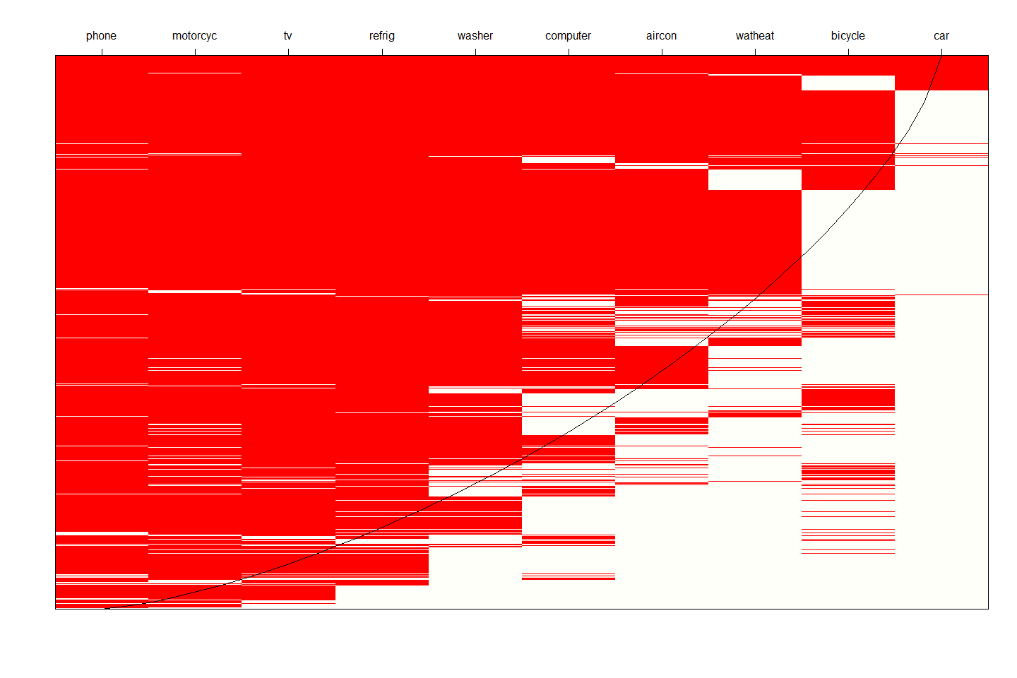

Code

## rearrange column follow the order of nestedness analysis 

wealth_index <- ipsum[,c("district","phone","motorcyc","tv","refrig",
                         "washer","computer","aircon","watheat",
                         "bicycle","car")] 

## select the highest property of each individual 
wealth_index <- cbind(wealth_index[,1],
                      wealth_index[,-1] %>%
                        rowwise() %>%
                        mutate(highest_property = names(.)[max(which(c_across(everything()) == 1))]) %>%
                        ungroup()) %>% na.omit()

wealth_index$quantile  <-  
           case_when(wealth_index$highest_property == "car" ~ "Richest, 25%",
                     wealth_index$highest_property == "bicycle" | 
                     wealth_index$highest_property == "watheat" | 
                     wealth_index$highest_property == "aircon"  ~ "Middle, 25%",
                     wealth_index$highest_property == "washer" | 
                     wealth_index$highest_property == "refrig"| 
                     wealth_index$highest_property == "computer"  ~ "Lower Middle, 25%",
                     wealth_index$highest_property == "phone" | 
                     wealth_index$highest_property == "motorcyc" | 
                     wealth_index$highest_property == "tv"   ~ "Poorest, 25%") %>% 
           factor(levels = c("Richest, 25%",
                             "Middle, 25%",
                             "Lower Middle, 25%",
                             "Poorest, 25%")
                    )

wealth <- wealth_index %>% group_by(district) %>% 
  count(quantile) %>% scale_per() %>% 
  mutate(dis = factor(district,
                      levels = as.character(sorted$district))) %>% 
  ggplot() +
  geom_col(aes(x = per,
               y = quantile)) +
  facet_wrap(vars(dis),
             # scales = "free",
             ncol = 1)+
  labs(x = "Percentage of total population(%)",
       y = "Wealth Quantile")+
  theme_light()+
  theme(axis.text.x = element_text(size = 15),
        axis.text.y = element_text(size = 15)) 

Code

vac_cov | time_vac | vac_dl | month_delay | wealth |edu | employ | reli | chil