install.packages(c("gtsummary", "broom.helpers"))Reproducible tables
Note
Dataset
library(gtsummary)
library(tidyverse)

df <- readRDS("../data/simulated_covid.rds")
First, let’s take a look at the data:
head(df) id case_name case_type sex age date_onset date_admission outcome
1 1 jCQH5RSlVq confirmed m 22 2023-01-01 <NA> recovered
2 2 AdCD3im7sn probable m 21 2023-01-08 <NA> recovered
3 3 iDzmfZhFkV probable m 21 2023-01-03 <NA> recovered
4 4 sKipHJsjZ2 probable m 10 2023-01-10 <NA> died
5 5 xG7GvAjlBf suspected m 24 2023-01-05 <NA> recovered
6 7 ZWWcBMLzoH confirmed m 10 2023-01-04 <NA> recovered
date_outcome date_first_contact date_last_contact district outbreak
1 <NA> <NA> <NA> Tan Binh 1st outbreak
2 <NA> 2022-12-31 2023-01-04 Tan Phu 1st outbreak
3 <NA> 2022-12-29 2023-01-05 Binh Tan 1st outbreak
4 2023-01-27 2023-01-10 2023-01-13 Quan 10 1st outbreak
5 <NA> 2023-01-07 2023-01-07 Quan 12 1st outbreak
6 <NA> 2023-01-06 2023-01-07 Binh Thanh 1st outbreak
Question
Is this data tidy?
The dataset is a line list, where each row represents a case with details such as sex, age, and outcome. This outbreak is interesting for its two distinct peaks. After a slight decrease in case counts in July, the numbers rose again.
Code
df %>%
  count(date_onset) %>%
  ggplot(
    aes(
      x = date_onset, y = n,
      text = paste0("Ngày: ", date_onset, "\n", "Số ca: ", n)
      )
    ) +
  geom_bar(stat = "identity", fill = "cornflowerblue") +
  labs(x = "Date of onset", y = "Case count") +
  theme_classic()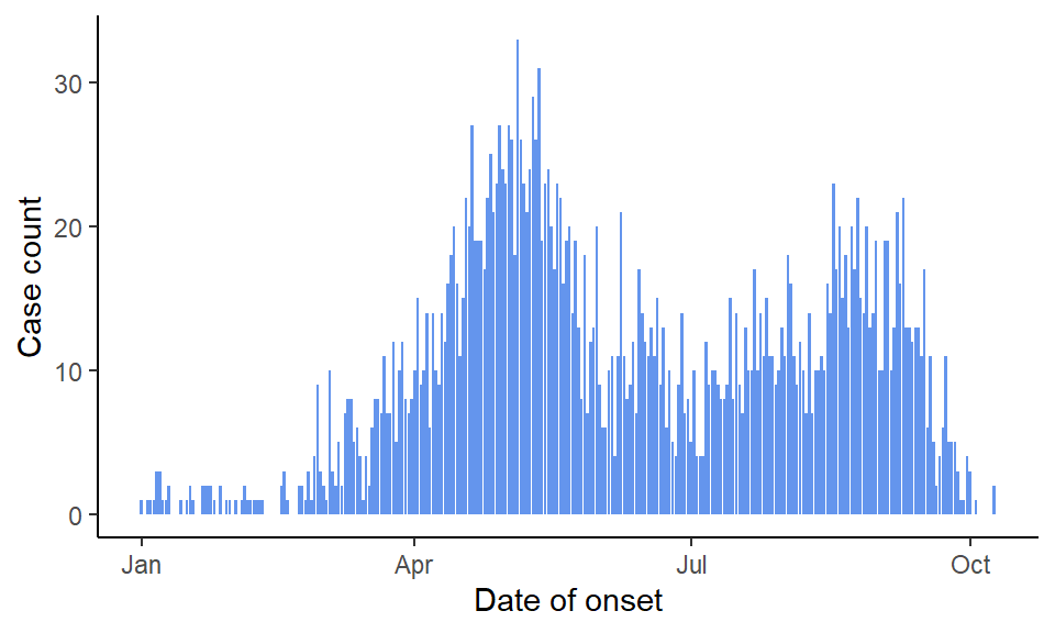
Descriptive tables
At the start of any analysis, it’s common to present a demographic table that summarises the characteristics of our sample. This can be done easily using tbl_summary() from the gtsummary package:
df %>%
  tbl_summary(
    include = c(sex, age, outcome, outbreak)
)| Characteristic | N = 2,7621 |
|---|---|
| sex | |
| f | 1,365 (49%) |
| m | 1,397 (51%) |
| age | 15 (8, 22) |
| outcome | |
| died | 220 (8.0%) |
| recovered | 2,542 (92%) |
| outbreak | |
| 1st outbreak | 1,513 (55%) |
| 2nd outbreak | 1,249 (45%) |
| 1 n (%); Median (Q1, Q3) | |
The variable labels and values in your table might not appear as expected. Let’s fix this, starting with the labels:
df %>%
  tbl_summary(
    include = c(sex, age, outcome, outbreak),
    label = list(sex ~ "Sex", age ~ "Age (years)", outcome ~ "Outcome", outbreak ~ "Outbreak")
)| Characteristic | N = 2,7621 |
|---|---|
| Sex | |
| f | 1,365 (49%) |
| m | 1,397 (51%) |
| Age (years) | 15 (8, 22) |
| Outcome | |
| died | 220 (8.0%) |
| recovered | 2,542 (92%) |
| Outbreak | |
| 1st outbreak | 1,513 (55%) |
| 2nd outbreak | 1,249 (45%) |
| 1 n (%); Median (Q1, Q3) | |
Now, let’s correct the values:
df %>%
  mutate(sex = factor(
    sex,
    levels = c("f", "m"),
    labels = c("Female", "Male")
  ),
  outcome = str_to_sentence(outcome)) %>%
  tbl_summary(
    include = c(sex, age, outcome, outbreak),
    label = list(sex ~ "Sex", age ~ "Age (years)", outcome ~ "Outcome", outbreak ~ "Outbreak")
)| Characteristic | N = 2,7621 |
|---|---|
| Sex | |
| Female | 1,365 (49%) |
| Male | 1,397 (51%) |
| Age (years) | 15 (8, 22) |
| Outcome | |
| Died | 220 (8.0%) |
| Recovered | 2,542 (92%) |
| Outbreak | |
| 1st outbreak | 1,513 (55%) |
| 2nd outbreak | 1,249 (45%) |
| 1 n (%); Median (Q1, Q3) | |
It looks pretty good now, but your supervisor mentioned that the number of decimals in your tables should be consistent. For example, percentages and continuous variables should both have one decimal place. Let’s fix that:
df %>%
  mutate(sex = factor(
    sex,
    levels = c("f", "m"),
    labels = c("Female", "Male")
  ),
  outcome = str_to_sentence(outcome)) %>%
  tbl_summary(
    include = c(sex, age, outcome, outbreak),
    label = list(sex ~ "Sex", age ~ "Age (years)", outcome ~ "Outcome", outbreak ~ "Outbreak"),
    digits = c(all_categorical() ~ c(0, 1), all_continuous() ~ 1)
)| Characteristic | N = 2,7621 |
|---|---|
| Sex | |
| Female | 1,365 (49.4%) |
| Male | 1,397 (50.6%) |
| Age (years) | 15.0 (8.0, 22.0) |
| Outcome | |
| Died | 220 (8.0%) |
| Recovered | 2,542 (92.0%) |
| Outbreak | |
| 1st outbreak | 1,513 (54.8%) |
| 2nd outbreak | 1,249 (45.2%) |
| 1 n (%); Median (Q1, Q3) | |
Okay, now the Age is displayed as the median with the quantile range, but your supervisor prefers it to be shown as the mean \(\pm\) standard deviation. Let’s change it:
df %>%
  mutate(sex = factor(
    sex,
    levels = c("f", "m"),
    labels = c("Female", "Male")
  ),
  outcome = str_to_sentence(outcome)) %>%
  tbl_summary(
    include = c(sex, age, outcome, outbreak),
    label = list(sex ~ "Sex", age ~ "Age (years)", outcome ~ "Outcome", outbreak ~ "Outbreak"),
    digits = c(all_categorical() ~ c(0, 1), all_continuous() ~ 1),
    statistic = list(
      all_continuous() ~ "{mean} \u00b1 {sd}"
    )
)| Characteristic | N = 2,7621 |
|---|---|
| Sex | |
| Female | 1,365 (49.4%) |
| Male | 1,397 (50.6%) |
| Age (years) | 15.5 ± 9.1 |
| Outcome | |
| Died | 220 (8.0%) |
| Recovered | 2,542 (92.0%) |
| Outbreak | |
| 1st outbreak | 1,513 (54.8%) |
| 2nd outbreak | 1,249 (45.2%) |
| 1 n (%); Mean ± SD | |
Extra tip for Vietnamese theses: Change the decimal mark from . to ,.
theme_gtsummary_language(language = "en", big.mark = ".", decimal.mark = ",")

df %>%
  mutate(sex = factor(
    sex,
    levels = c("f", "m"),
    labels = c("Female", "Male")
  ),
  outcome = str_to_sentence(outcome)) %>%
  tbl_summary(
    include = c(sex, age, outcome, outbreak),
    label = list(sex ~ "Sex", age ~ "Age (years)", outcome ~ "Outcome", outbreak ~ "Outbreak"),
    digits = c(all_categorical() ~ c(0, 1), all_continuous() ~ 1),
    statistic = list(
      all_continuous() ~ "{mean} \u00b1 {sd}"
    )
)| Characteristic | N = 2.7621 |
|---|---|
| Sex | |
| Female | 1.365 (49,4%) |
| Male | 1.397 (50,6%) |
| Age (years) | 15,5 ± 9,1 |
| Outcome | |
| Died | 220 (8,0%) |
| Recovered | 2.542 (92,0%) |
| Outbreak | |
| 1st outbreak | 1.513 (54,8%) |
| 2nd outbreak | 1.249 (45,2%) |
| 1 n (%); Mean ± SD | |
Statistical inference
The most common goal is to compare two groups and make inferences. In gtsummary, you can do this by simply copying the code for the descriptive table and adding the by = group_variable argument. Just remember to remove the group_variable from include if you included it in the descriptive table.
df %>%
  mutate(sex = factor(
    sex,
    levels = c("f", "m"),
    labels = c("Female", "Male")
  ),
  outcome = str_to_sentence(outcome)) %>%
  tbl_summary(
    by = outbreak,
    include = c(sex, age, outcome),
    label = list(sex ~ "Sex", age ~ "Age (years)", outcome ~ "Outcome"),
    digits = c(all_categorical() ~ c(0, 1), all_continuous() ~ 1),
    statistic = list(
      all_continuous() ~ "{mean} \u00b1 {sd}"
    )
)| Characteristic | 1st outbreak N = 1,5131 |
2nd outbreak N = 1,2491 |
|---|---|---|
| Sex | ||
| Female | 746 (49.3%) | 619 (49.6%) |
| Male | 767 (50.7%) | 630 (50.4%) |
| Age (years) | 12.8 ± 7.6 | 18.8 ± 9.6 |
| Outcome | ||
| Died | 110 (7.3%) | 110 (8.8%) |
| Recovered | 1,403 (92.7%) | 1,139 (91.2%) |
| 1 n (%); Mean ± SD | ||
Look good now! You probably need p-values. Add them using the add_p() function.
df %>%
  mutate(sex = factor(
    sex,
    levels = c("f", "m"),
    labels = c("Female", "Male")
  ),
  outcome = str_to_sentence(outcome)) %>%
  tbl_summary(
    by = outbreak,
    include = c(sex, age, outcome),
    label = list(sex ~ "Sex", age ~ "Age (years)", outcome ~ "Outcome"),
    digits = c(all_categorical() ~ c(0, 1), all_continuous() ~ 1),
    statistic = list(
      all_continuous() ~ "{mean} \u00b1 {sd}"
    )
  ) %>%
add_p()| Characteristic | 1st outbreak N = 1,5131 |
2nd outbreak N = 1,2491 |
p-value2 |
|---|---|---|---|
| Sex | 0.9 | ||
| Female | 746 (49.3%) | 619 (49.6%) | |
| Male | 767 (50.7%) | 630 (50.4%) | |
| Age (years) | 12.8 ± 7.6 | 18.8 ± 9.6 | <0.001 |
| Outcome | 0.14 | ||
| Died | 110 (7.3%) | 110 (8.8%) | |
| Recovered | 1,403 (92.7%) | 1,139 (91.2%) | |
| 1 n (%); Mean ± SD | |||
| 2 Pearson’s Chi-squared test; Wilcoxon rank sum test | |||
Again, your supervisor wants p-values displayed with three decimal digits. Let do it:
df %>%
  mutate(sex = factor(
    sex,
    levels = c("f", "m"),
    labels = c("Female", "Male")
  ),
  outcome = str_to_sentence(outcome)) %>%
  tbl_summary(
    by = outbreak,
    include = c(sex, age, outcome),
    label = list(sex ~ "Sex", age ~ "Age (years)", outcome ~ "Outcome"),
    digits = c(all_categorical() ~ c(0, 1), all_continuous() ~ 1),
    statistic = list(all_continuous() ~ "{mean} \u00b1 {sd}")
  ) %>%
  add_p(
    pvalue_fun = function(x)
      style_pvalue(x, digits = 3)
)| Characteristic | 1st outbreak N = 1,5131 |
2nd outbreak N = 1,2491 |
p-value2 |
|---|---|---|---|
| Sex | 0.894 | ||
| Female | 746 (49.3%) | 619 (49.6%) | |
| Male | 767 (50.7%) | 630 (50.4%) | |
| Age (years) | 12.8 ± 7.6 | 18.8 ± 9.6 | <0.001 |
| Outcome | 0.138 | ||
| Died | 110 (7.3%) | 110 (8.8%) | |
| Recovered | 1,403 (92.7%) | 1,139 (91.2%) | |
| 1 n (%); Mean ± SD | |||
| 2 Pearson’s Chi-squared test; Wilcoxon rank sum test | |||
You discovered that the default test is the Wilcoxon test, but now you want to use the t-test for age. Specify it in add_p() like this:
df %>%
  mutate(sex = factor(
    sex,
    levels = c("f", "m"),
    labels = c("Female", "Male")
  ),
  outcome = str_to_sentence(outcome)) %>%
  tbl_summary(
    by = outbreak,
    include = c(sex, age, outcome),
    label = list(sex ~ "Sex", age ~ "Age (years)", outcome ~ "Outcome"),
    digits = c(all_categorical() ~ c(0, 1), all_continuous() ~ 1),
    statistic = list(all_continuous() ~ "{mean} \u00b1 {sd}")
  ) %>%
  add_p(
    pvalue_fun = function(x)
      style_pvalue(x, digits = 3),
    test = list(age ~ "t.test")
)| Characteristic | 1st outbreak N = 1,5131 |
2nd outbreak N = 1,2491 |
p-value2 |
|---|---|---|---|
| Sex | 0.894 | ||
| Female | 746 (49.3%) | 619 (49.6%) | |
| Male | 767 (50.7%) | 630 (50.4%) | |
| Age (years) | 12.8 ± 7.6 | 18.8 ± 9.6 | <0.001 |
| Outcome | 0.138 | ||
| Died | 110 (7.3%) | 110 (8.8%) | |
| Recovered | 1,403 (92.7%) | 1,139 (91.2%) | |
| 1 n (%); Mean ± SD | |||
| 2 Pearson’s Chi-squared test; Welch Two Sample t-test | |||
We’re nearly there. Your supervisor (yet again) wants an overall column. Simply add it using add_overall():
df %>%
  mutate(sex = factor(
    sex,
    levels = c("f", "m"),
    labels = c("Female", "Male")
  ),
  outcome = str_to_sentence(outcome)) %>%
  tbl_summary(
    by = outbreak,
    include = c(sex, age, outcome),
    label = list(sex ~ "Sex", age ~ "Age (years)", outcome ~ "Outcome"),
    digits = c(all_categorical() ~ c(0, 1), all_continuous() ~ 1),
    statistic = list(all_continuous() ~ "{mean} \u00b1 {sd}")
  ) %>%
  add_p(
    pvalue_fun = function(x)
      style_pvalue(x, digits = 3),
    test = list(age ~ "t.test")
  ) %>%
add_overall()| Characteristic | Overall N = 2,7621 |
1st outbreak N = 1,5131 |
2nd outbreak N = 1,2491 |
p-value2 |
|---|---|---|---|---|
| Sex | 0.894 | |||
| Female | 1,365 (49.4%) | 746 (49.3%) | 619 (49.6%) | |
| Male | 1,397 (50.6%) | 767 (50.7%) | 630 (50.4%) | |
| Age (years) | 15.5 ± 9.1 | 12.8 ± 7.6 | 18.8 ± 9.6 | <0.001 |
| Outcome | 0.138 | |||
| Died | 220 (8.0%) | 110 (7.3%) | 110 (8.8%) | |
| Recovered | 2,542 (92.0%) | 1,403 (92.7%) | 1,139 (91.2%) | |
| 1 n (%); Mean ± SD | ||||
| 2 Pearson’s Chi-squared test; Welch Two Sample t-test | ||||
Great! Finally, we usually highlight small p-values to guide readers to the exciting findings. Just use bold_p() and set the threshold you want:
df %>%
  mutate(sex = factor(
    sex,
    levels = c("f", "m"),
    labels = c("Female", "Male")
  ),
  outcome = str_to_sentence(outcome)) %>%
  tbl_summary(
    by = outbreak,
    include = c(sex, age, outcome),
    label = list(sex ~ "Sex", age ~ "Age (years)", outcome ~ "Outcome"),
    digits = c(all_categorical() ~ c(0, 1), all_continuous() ~ 1),
    statistic = list(all_continuous() ~ "{mean} \u00b1 {sd}")
  ) %>%
  add_p(
    pvalue_fun = function(x)
      style_pvalue(x, digits = 3),
    test = list(age ~ "t.test")
  ) %>%
  add_overall() %>%
bold_p(t = 0.05)| Characteristic | Overall N = 2,7621 |
1st outbreak N = 1,5131 |
2nd outbreak N = 1,2491 |
p-value2 |
|---|---|---|---|---|
| Sex | 0.894 | |||
| Female | 1,365 (49.4%) | 746 (49.3%) | 619 (49.6%) | |
| Male | 1,397 (50.6%) | 767 (50.7%) | 630 (50.4%) | |
| Age (years) | 15.5 ± 9.1 | 12.8 ± 7.6 | 18.8 ± 9.6 | <0.001 |
| Outcome | 0.138 | |||
| Died | 220 (8.0%) | 110 (7.3%) | 110 (8.8%) | |
| Recovered | 2,542 (92.0%) | 1,403 (92.7%) | 1,139 (91.2%) | |
| 1 n (%); Mean ± SD | ||||
| 2 Pearson’s Chi-squared test; Welch Two Sample t-test | ||||
Univariate analysis
The next step in a typical analysis is to perform a univariate analysis and calculate the odds ratio (OR) for each variable:
df %>%
  mutate(sex = factor(
    sex,
    levels = c("f", "m"),
    labels = c("Female", "Male")
  ),
  outcome = str_to_sentence(outcome)) %>%
  tbl_uvregression(
    method = glm,
    y = outbreak,
    method.args = list(family = binomial),
    exponentiate = TRUE,
    include = c(sex, age, outcome),
    label = list(sex ~ "Sex", age ~ "Age (years)", outcome ~ "Outcome"),
    pvalue_fun = function(x)
      style_pvalue(x, digits = 3)
  ) %>%
bold_p(t = 0.05)| Characteristic | N | OR | 95% CI | p-value |
|---|---|---|---|---|
| Sex | 2,762 | |||
| Female | — | — | ||
| Male | 0.99 | 0.85 – 1.15 | 0.894 | |
| Age (years) | 2,762 | 1.08 | 1.07 – 1.09 | <0.001 |
| Outcome | 2,762 | |||
| Died | — | — | ||
| Recovered | 0.81 | 0.62 – 1.07 | 0.138 | |
| Abbreviations: CI = Confidence Interval, OR = Odds Ratio | ||||
If you want to hide the sample size, add hide_n = TRUE:
df %>%
  mutate(sex = factor(
    sex,
    levels = c("f", "m"),
    labels = c("Female", "Male")
  ),
  outcome = str_to_sentence(outcome)) %>%
  tbl_uvregression(
    method = glm,
    y = outbreak,
    method.args = list(family = binomial),
    exponentiate = TRUE,
    hide_n = TRUE,
    include = c(sex, age, outcome),
    label = list(sex ~ "Sex", age ~ "Age (years)", outcome ~ "Outcome"),
    pvalue_fun = function(x)
      style_pvalue(x, digits = 3)
  ) %>%
bold_p(t = 0.05)| Characteristic | OR | 95% CI | p-value |
|---|---|---|---|
| Sex | |||
| Female | — | — | |
| Male | 0.99 | 0.85 – 1.15 | 0.894 |
| Age (years) | 1.08 | 1.07 – 1.09 | <0.001 |
| Outcome | |||
| Died | — | — | |
| Recovered | 0.81 | 0.62 – 1.07 | 0.138 |
| Abbreviations: CI = Confidence Interval, OR = Odds Ratio | |||
Multivariate analysis
Finally, you might want to run a multivariate analysis to adjust these OR values for confounders:
df %>%
  mutate(sex = factor(
    sex,
    levels = c("f", "m"),
    labels = c("Female", "Male")
  ),
  outcome = str_to_sentence(outcome)) %>%
  glm(outbreak ~ sex + age + outcome, data = ., family = binomial) %>%
  tbl_regression(
    exponentiate = TRUE,
    label = list(sex ~ "Sex", age ~ "Age (years)", outcome ~ "Outcome"),
    pvalue_fun = function(x)
      style_pvalue(x, digits = 3)
  ) %>%
bold_p(t = 0.05)| Characteristic | OR | 95% CI | p-value |
|---|---|---|---|
| Sex | |||
| Female | — | — | |
| Male | 0.98 | 0.84 – 1.15 | 0.824 |
| Age (years) | 1.08 | 1.07 – 1.09 | <0.001 |
| Outcome | |||
| Died | — | — | |
| Recovered | 0.85 | 0.63 – 1.13 | 0.265 |
| Abbreviations: CI = Confidence Interval, OR = Odds Ratio | |||