4  Manuscript figure

Code
library(readxl)
library(tidyverse)
library(gtsummary)
library(patchwork)
library(lubridate)
library(stringr)
library(mgcv)
library(janitor)
library(predtools)
library(magrittr)
library(slider)
library(scam)
library(epitools)
library(sf)
library(stringi)
invisible(Sys.setlocale("LC_TIME", "English"))
Code
## data import

## case notification
df1 <- read_excel("D:/OUCRU/hfmd/data/TCM_full.xlsx",
                  col_types = c("date", "numeric", "text",
                                "text", "text", "date", "date", "date",
                                "text", "text", "text"))
colnames(df1) <- c("dob", "age", "gender", "commune", "district",
                   "reported_date", "onset_date","adm_date",
                   "medi_cen","inout","severity")
df1$dob <- df1$dob %>% as_date()
df1$adm_date <- df1$adm_date %>% as_date()

df1$age1 <- interval(df1$dob, df1$adm_date) / years(1)
df1$adm_week <- as.Date(floor_date(df1$adm_date, "week"))
df1$district <- df1$district %>% str_replace_all(
  c( "Quận Gò vấp"  = "Quận Gò Vấp"))
df1$district <- df1$district %>%
  str_remove("Quận|Huyện|Thành phố") %>%
  trimws(which = "both")

## serological data

apr_2023 <- read_excel("D:/OUCRU/hfmd/data/4_2023.xlsx")
aug_2023 <- read_excel("D:/OUCRU/hfmd/data/08_2023.xlsx")
dec_2022 <- read_excel("D:/OUCRU/hfmd/data/12_2022.xls")
dec_2023 <- read_excel("D:/OUCRU/hfmd/data/12_2023.xlsx")

t423 <- data.frame(apr_2023[-c(1,2),c(6,8,10:14)])
t423$pos <- replace(t423$...14,is.na(t423$...14),0) %>%
  str_detect(regex(paste(2^(4:10), collapse = "|"))) %>%
  as.integer(as.logical())
colnames(t423) <- c("id","age_gr","age","col_day","col_month","col_year","neutralization","pos")
t423$age <- as.numeric(t423$age)
t423$col_time <- rep("Apr 2023",nrow(t423))


t823 <- data.frame(aug_2023[-c(1,2),c(6,8,9,14:17)])
t823$pos <- str_detect(t823$...17,regex(paste(2^(4:10), collapse = "|"))) %>%
  as.integer(as.logical())
colnames(t823) <- c("id","age_gr","age","col_day","col_month","col_year","neutralization","pos")
t823$age <- as.numeric(t823$age)
t823$col_time <- rep("Aug 2023",nrow(t823))

t1222 <- data.frame(dec_2022[-c(1,2),c(6,8,10:14)])
t1222$pos <- replace(t1222$...14,is.na(t1222$...14),0) %>%
  str_detect(regex(paste(2^(4:10), collapse = "|"))) %>%
  as.integer(as.logical())
colnames(t1222) <- c("id","age_gr","age","col_day","col_month","col_year","neutralization","pos")
t1222$age <- as.numeric(t1222$age)
t1222$col_time <- rep("Dec 2022",nrow(t1222))


t1223 <- data.frame(dec_2023[-c(1,2),c(6,8,9,14:17)])
t1223$pos <- replace(t1223$...17,is.na(t1223$...17),0) %>%
  str_detect(regex(paste(2^(4:10), collapse = "|"))) %>%
  as.integer(as.logical())
colnames(t1223) <- c("id","age_gr","age","col_day","col_month","col_year","neutralization","pos")
t1223$age <- as.numeric(t1223$age)
t1223$col_time <- rep("Dec 2023",nrow(t1223))

## data sero with address

cleaned <- read_csv("D:/OUCRU/HCDC/project phân tích sero quận huyện/cleaned.csv")

sero <- rbind(t1222,t1223,t423,t823)

sero_add <- full_join(cleaned,sero, by =  c("id" = "id"))

data_pt <- sero_add %>% filter(!is.na(age)&!is.na(qhchuan)) %>%
  dplyr::select(-c(add_mod,pxchuan,neutralization)) %>%
  as.data.frame() %>% 
  mutate(col_date = make_date(col_year,col_month,col_day))

## census data

census2019 <- readRDS("D:/OUCRU/hfmd/data/census2019.rds")

### HCMC map
map_path <- "D:/OUCRU/HCDC/project phân tích sero quận huyện/"
vn_qh <- st_read(dsn = file.path(map_path, "gadm41_VNM.gpkg"), layer = "ADM_ADM_2")

vn_qh1 <- vn_qh %>%
  clean_names() %>%     ## cho thành chữ thường
  filter(
    str_detect(
      name_1,
      "Hồ Chí Minh"
    )
  )
qhtp <- vn_qh1[-c(14,21),]

qhtp$geom[qhtp$varname_2 == "Thu Duc"] <- vn_qh1[c("21","24","14"),] %>%
  st_union()

qhtp <- qhtp %>% st_cast("MULTIPOLYGON")

qhtp$varname_2 <- stri_trans_general(qhtp$varname_2, "latin-ascii") %>%
  tolower() %>%
  str_remove("district") %>%
  trimws(which = "both")

qhtp$nl_name_2 <- c("BC","BTân","BT","CG","CC","GV",
                    "HM","NB","PN","1","10","11","12",
                    "3","4","5","6","7","8","TB",
                    "TP","TĐ")
Code
# function

slide_age <- function(time1,age1,w1,s1){
  df1 <- data.frame(time1,age1) %>%                   ## line listing data frame
    filter(!is.na(time1) & !is.na(age1)) %>%
    arrange(time1)

  a_df1 <- df1 %>% count(time1)                      ## aggregate data frame

  total1 <- nrow(a_df1)
  spots1 <- seq(from = 1, to = (total1 - w1 + 1), by = s1)

  out_total <- data.frame()

  for (i in 1:length(spots1)){
    range1 <- data.frame(a_df1[spots1[i]:(spots1[i] + w1 - 1),1])
    result1 <- df1$age1[df1$time1 >= range1[1,] & df1$time1 <= range1[w1,]]
    out <- data.frame(date = rep(as.character(range1[ceiling(w1/2),]),length(result1)),
                      age = result1)
    out <- out[order(out$age),]
    out_total <- rbind(out_total,out)
  }
  output <- list()
  output$wdat <- out_total
  output$adat <- out_total %>% count(date)
  output$parms <- data.frame(w = w1,s =s1)
  return(output)
}


# case_noti <- function(timee, agee,lab = FALSE){
# 
#   dat <- data.frame(timee,agee) %>%
#     filter(!is.na(timee) & !is.na(agee)) %>%
#     count(timee)
# 
#   ts <- ggplot(dat, aes(x =timee, y = n)) +
#     geom_bar(stat = "identity") +
#     labs(y = "Cases") +
#     theme_minimal()
# 
#   if(lab == TRUE){
#     ts
#   } else {
#     ts + theme(axis.title.x = element_blank(),
#                axis.text.x = element_blank(),
#                axis.ticks.x = element_blank())
#   }
# 
# }

4.1 Figure 1: heat map

Code
library(paletteer)
df23 <- df1 %>% filter(year(adm_week) == 2023)

co <- data.frame()

for (i in 0:6){
  gen <- seq(0,1,le=52) + i
  co <- rbind(co,gen)
}


df23 <- df1 %>% filter(year(adm_date) == 2023)
wwww <- slide_age(time1 = df23$adm_date,
                  age1 =  df23$age1,
                  w1 = 7, s1=7)

library(zoo)
ch <- data.frame(date = wwww$adat$date,
                 c0 = as.numeric(co[1,]),
                 c1 = as.numeric(co[2,]),
                 c2 = as.numeric(co[3,]),
                 c3 = as.numeric(co[4,]),
                 c4 = as.numeric(co[5,]),
                 c5 = as.numeric(co[6,]))

ch <- ch %>% mutate(
  trend = c(rep("#80FFFFFF",26-3),
            rep("#FFFFFFFF",26+3))
)

ch$group <- consecutive_id(ch$trend)
ch <- head(do.call(rbind, by(ch, ch$group, rbind, NA)), -1)
ch[, c("trend", "group")] <- lapply(ch[, c("trend", "group")], na.locf)
ch[] <- lapply(ch, na.locf, fromLast = T)

ch$trend <- factor(ch$trend,
                   levels = c("#80FFFFFF","#FFFFFFFF"))

leb_month <- c("Jan",rep("",3),"Feb",rep("",3),"Mar",rep("",4),"Apr",rep("",3),
               "May",rep("",4),"Jun",rep("",3),"Jul",rep("",3),"Aug",rep("",4),
               "Sep",rep("",3),"Oct",rep("",3),"Nov",rep("",4),"Dec",rep("",3))

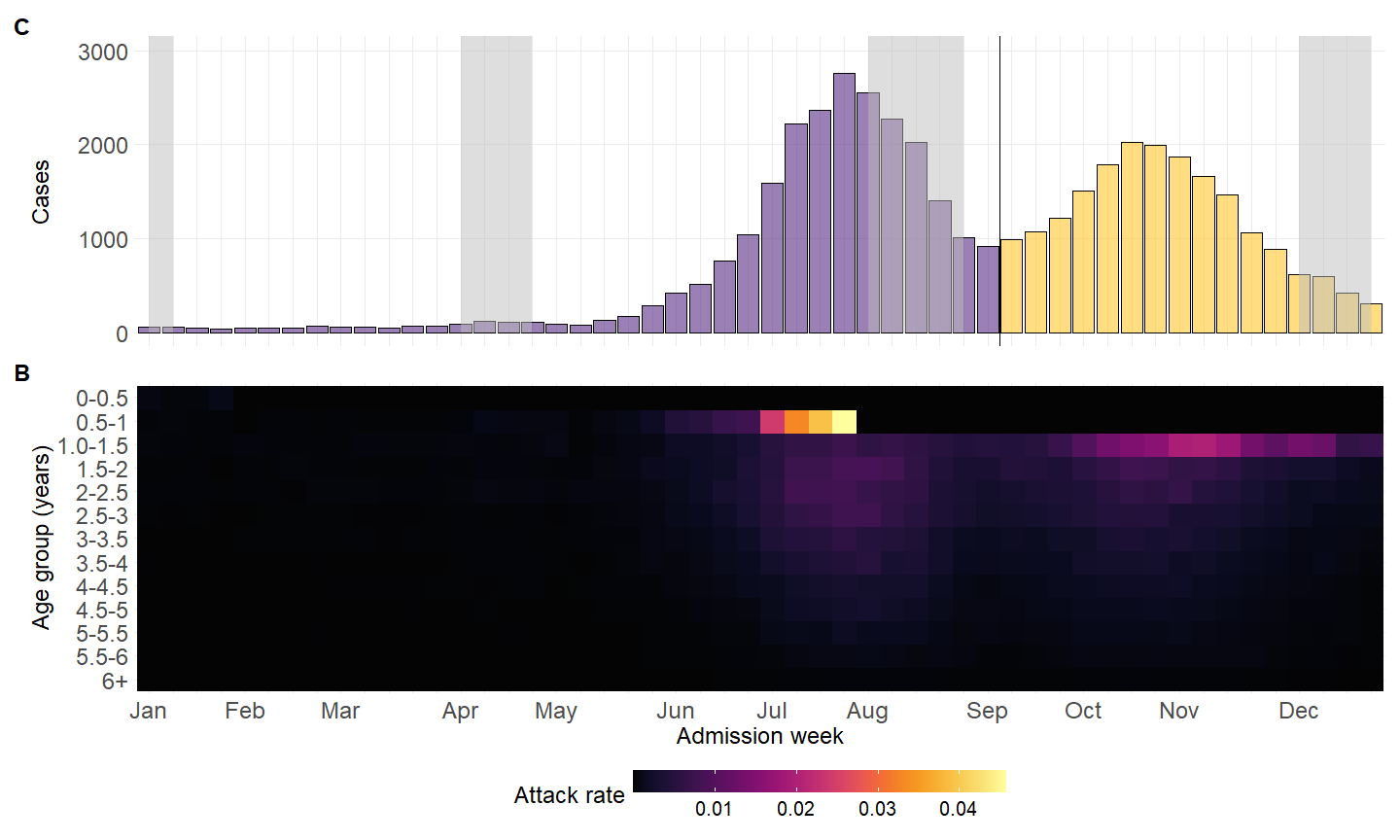
ts <- data.frame(wwww$wdat$date,wwww$wdat$age) %>%
  filter(!is.na(wwww$wdat$date) & !is.na(wwww$wdat$age)) %>%
  count(wwww$wdat$date) %>%
  set_colnames(c("time","n")) %>% 
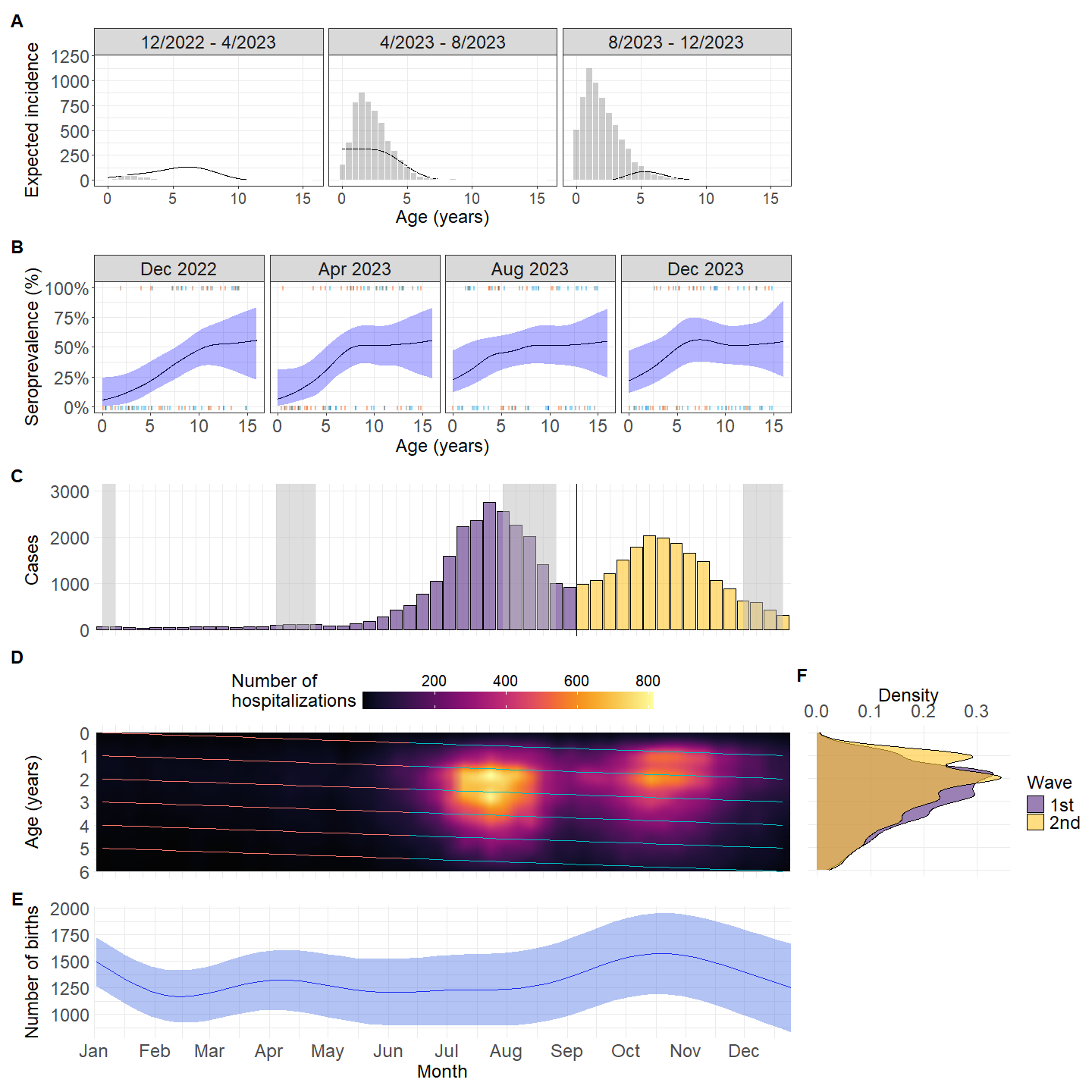
  mutate(peak = c(rep("1st",36),rep("2nd",nrow(.)-36))) %>% 
  ggplot(aes(x = time, y = n,fill = peak)) +
  geom_col(alpha = 0.6,color="black") +
  geom_vline(xintercept = 36.5) +
  theme_minimal()+
  scale_y_continuous(name = "Cases",
                     breaks = seq(0,3000,by = 1000),
                     limit =c(0,3000), 
                     minor_breaks = NULL)+
  scale_fill_manual(values = c("#582C83FF","#FFC72CFF"))+
  labs(tag = "C")+ 
  annotate("rect", fill = "grey",
           xmin = c("2023-01-04","2023-04-05","2023-08-02","2023-12-06"), 
           xmax = c("2023-01-11","2023-04-26","2023-08-30","2023-12-27"), 
           ymin = 0, ymax = Inf, alpha = .5)+
  theme(axis.title.x = element_blank(),
        axis.text.x = element_blank(),
        axis.ticks.x = element_blank(),
        legend.position = "none",
        plot.tag = element_text(face = "bold", size = 18),
        axis.title.y = element_text(size = 18),
        axis.text.y = element_text(size = 18))

hm <- ggplot(data=wwww$wdat, aes(x=date, y=age)) +
  stat_density(
    aes(fill = after_stat(density)),
    geom = "raster",
    position = "identity",
    interpolate = TRUE
  )+
  scale_fill_paletteer_c("grDevices::Inferno")+
  # scale_fill_gradient(low="#040404FF", high= "#FFFE9EFF")+
  # scale_fill_distiller(palette = "Blues")+
  theme_minimal()+
  scale_y_reverse(name = "Age (years)",lim= rev(c(0,6)),breaks = seq(0,6))+
  scale_x_discrete(name = "Admission week",labels = leb_month)+
  labs(tag = "D",fill = "Density")+
  # theme(axis.text.x = element_text(angle = 90, vjust = 0.5, hjust=1,size = 8))+
  geom_line(data = ch,aes(x = date,y = c0,col = trend),
            group = 1,lwd = 0.25)+
  geom_line(data = ch,aes(x = date,y = c1,col = trend),
            group = 1,lwd = 0.25)+
  geom_line(data = ch,aes(x = date,y = c2,col = trend),
            group = 1,lwd = 0.25)+
  geom_line(data = ch,aes(x = date,y = c3,col = trend),
            group = 1,lwd = 0.25)+
  geom_line(data = ch,aes(x = date,y = c4,col = trend),
            group = 1,lwd = 0.25)+
  geom_line(data = ch,aes(x = date,y = c5,col = trend),
            group = 1,lwd = 0.25)+
  theme(axis.title.y = element_text(size = 18),
        axis.title.x = element_blank(),
        axis.ticks.x = element_blank(),
        legend.position = "top",
        plot.tag = element_text(face = "bold", size = 18),
        axis.text.x = element_blank(),
        axis.text.y = element_text(size = 18),
        legend.text = element_text(size = 15),
        legend.title = element_text(size = 18))+ 
  guides(fill=guide_colourbar(barwidth=20,
                              label.position="top"),
         color = "none") 


hm2 <- ggplot(data=wwww$wdat, aes(x=date, y=age)) +
  stat_density(
    aes(fill = after_stat(count)),
    geom = "raster",
    position = "identity",
    interpolate = TRUE
  )+
  scale_fill_paletteer_c("grDevices::Inferno")+
  # scale_fill_gradient(low="#040404FF", high= "#FFFE9EFF")+
  # scale_fill_distiller(palette = "Blues")+
  theme_minimal()+
  scale_y_reverse(name = "Age (years)",lim= rev(c(0,6)),breaks = seq(0,6))+
  scale_x_discrete(name = "Admission week",labels = leb_month)+
  labs(tag = "D",fill = "Number of hospitalizations")+
  # theme(axis.text.x = element_text(angle = 90, vjust = 0.5, hjust=1,size = 8))+
  geom_line(data = ch,aes(x = date,y = c0,col = trend),
            group = 1,lwd = 0.25)+
  geom_line(data = ch,aes(x = date,y = c1,col = trend),
            group = 1,lwd = 0.25)+
  geom_line(data = ch,aes(x = date,y = c2,col = trend),
            group = 1,lwd = 0.25)+
  geom_line(data = ch,aes(x = date,y = c3,col = trend),
            group = 1,lwd = 0.25)+
  geom_line(data = ch,aes(x = date,y = c4,col = trend),
            group = 1,lwd = 0.25)+
  geom_line(data = ch,aes(x = date,y = c5,col = trend),
            group = 1,lwd = 0.25)+
  theme(axis.title.y = element_text(size = 18),
        axis.title.x = element_blank(),
        axis.ticks.x = element_blank(),
        legend.position = "top",
        plot.tag = element_text(face = "bold", size = 18),
        axis.text.x = element_blank(),
        axis.text.y = element_text(size = 18),
        legend.text = element_text(size = 15),
        legend.title = element_text(size = 18))+ 
  guides(fill=guide_colourbar(barwidth=20,
                              label.position="top"),
         color = "none")


fi_peak <- df1 %>% filter(year(adm_date) == "2023") %>%
  filter((adm_date <= as.Date("2023-09-03")&
            !is.na(adm_date) & !is.na(age1)))

se_peak <- df1 %>% filter(year(adm_date) == "2023") %>%
  filter((adm_date > as.Date("2023-09-03")) &
           !is.na(adm_date) & !is.na(age1))

data <- data.frame(
  peak = c( rep("1st",nrow(data.frame(se_peak$age1))),
            rep("2nd",nrow(data.frame(fi_peak$age1)))),
  age = c( fi_peak$age1, se_peak$age1 )
)

## density plot

ad <- ggplot(data=data, aes(x=age, group=peak, fill=peak)) +
  geom_density(alpha = 0.6) +
  scale_fill_manual(values = c("#582C83FF","#FFC72CFF")) +
  scale_x_reverse(limit = c(6,0),
                  breaks = seq(0,6,by=1), 
                  minor_breaks = NULL)+
  scale_y_continuous(minor_breaks = NULL,position = "right")+
  coord_flip()+
  theme_minimal()+
  labs(x = "Age", y ="Density",tag = "F",fill = "Wave")+
  theme(axis.title.y = element_blank(),
        axis.ticks.x = element_blank(),
        # legend.position = "top",
        plot.tag = element_text(face = "bold", size = 18),
        axis.title.x = element_text(size = 18),
        axis.text.x = element_text(size = 18),
        axis.text.y = element_blank(),
        legend.text = element_text(size = 18),
        legend.title = element_text(size = 18))


library(ISOweek)
count_dangky_week <- readRDS("D:/OUCRU/hfmd/data/count_dangky_week.rds")
child <- count_dangky_week %>% filter(birth_year >= 2017) %>% group_by(birth_week, birth_year) %>%
  summarise(n=sum(n)) %>% arrange(birth_year)
colnames(child) <- c("week","year","birth")
## combine week 52 and 53

child$week <- ifelse(child$week == 53,52,child$week)

child <- child %>% group_by(year) %>%
  mutate(newn = ifelse(week == 52, sum(birth[week==52]), birth)) %>%
  {data.frame(.$week, .$year, .$newn )} %>% unique() %>%
  magrittr::set_colnames(c("week","year","birth"))

child$week2 <- seq(1:length(child$week))

time <- data.frame()

for (i in 2017:2022){
  range <- child$week[child$year == i]
  if (length(range) == 52){
    time_add <- seq.int(i + 7/365 ,(i+1) - 7/365,
                        length.out = length(range)) %>% data.frame()
  } else {
    time_add <- seq.int(i + 7/365 ,(i+1) - 7/365,
                        length.out = 52)[1:length(range)] %>% data.frame()
  }
  time <- rbind(time,time_add)
}


child[,5] <- time %>%
  magrittr::set_colnames(c("time"))

## model fitting
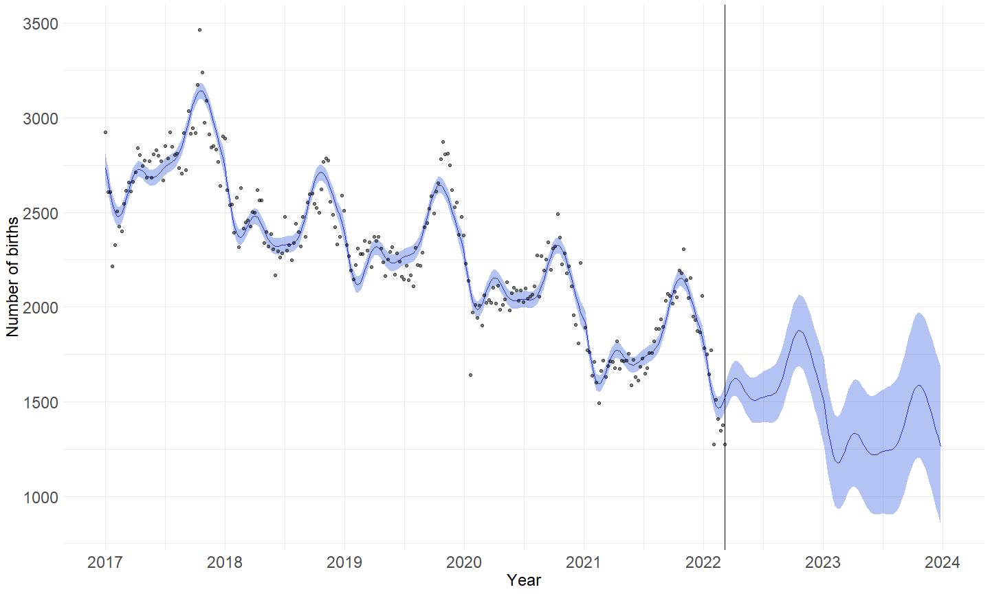
fit <- mgcv::gam(birth ~ s(week) + s(week2),method = "REML",data = child)


cutpoint <- function(point){
  fitt <- mgcv::gam(birth ~ s(week) + s(week2),
                    method = "REML",data = child[-c(point:nrow(child)),])
  
  new_data2 <- data.frame(week = rep(1:52,7))
  
  new_data2$week2 <- seq(1,nrow(new_data2))
  new_data2$year <- rep(2017:2023,each = 52)
  
  time <- data.frame()
  for (i in 2017:2023){
    range <- new_data2$week[new_data2$year == i]
    time_add <- data.frame(seq.int(i + 7/365 ,(i+1) - 7/365,
                                   length.out = length(range)))
    time <- rbind(time,time_add)
  }
  
  new_data2[4] <- time %>%
    magrittr::set_colnames(c("time"))
  
  est2 <- predict.gam(fitt,newdata = new_data2,
                      type="response",se.fit = TRUE)
  
  new_data2 <- new_data2 %>% mutate(
    fit = est2$fit,
    lwr = est2$fit - qt(0.95,nrow(new_data2))*est2$se.fit,
    upr = est2$fit + qt(0.95,nrow(new_data2))*est2$se.fit,
  )
  out <- list()
  out$point <- point
  out$df <- new_data2
  return(out)
}


plot_cp <- function(model){
  dta <- model$df %>% 
    mutate(time2 = sprintf("%04d-W%02d-1", year, week),
           time2 = ISOweek2date(time2)) 
  ggplot(data = dta) +
    geom_line(aes(x = time2,y = fit),col = "blue")+
    geom_ribbon(aes(x = time2,ymin = lwr, ymax = upr), fill = "royalblue",alpha = 0.4)+
    geom_vline(xintercept = dta$time2[dta$week2 == model$point])+
    labs(y = "Number of births",
         x = "Year")+
    theme_minimal()
}


model <- cutpoint(270)

b_ss <- plot_cp(model)+
  geom_point(data = child[1:270,]%>% 
               mutate(time2 = sprintf("%04d-W%02d-1", year, week),
                      time2 = ISOweek2date(time2)) , 
             aes(x = time2, y = birth),alpha = 0.5)+
  # annotate("text", x= 2017, y=3500, label= "Fitting") +
  # annotate("text", x = 2023.5, y=3500, label = "Estimation")+
  scale_x_date(date_labels = "%Y",
               breaks = seq(as.Date("2017-01-01"),
                                 as.Date("2024-01-01"),
                                 by = "1 year"),
               limits = c(as.Date("2017-01-01"),
                          as.Date("2024-01-01")))+
  theme(axis.title.y = element_text(size = 18),
        axis.ticks.x = element_blank(),
        legend.position = "bottom",
        plot.tag = element_text(face = "bold", size = 18),
        axis.title.x = element_text(size = 18),
        axis.text.x = element_text(size = 18),
        axis.text.y = element_text(size = 18),
        legend.text = element_text(size = 15),
        legend.title = element_text(size = 18))
Code
library(nortest)
ks.test(age~peak,data = data,altervative = "two.sided")

    Asymptotic two-sample Kolmogorov-Smirnov test

data:  age by peak
D = 0.083993, p-value < 2.2e-16
alternative hypothesis: two-sided

4.1.1 Age distribution of raw data

Code
library(fitdistrplus)
fit1 <- fitdist(fi_peak %>% filter(age1 >0) %>% pull(age1),"lnorm")
fit2 <- fitdist(se_peak %>% filter(age1 >0) %>% pull(age1),"lnorm")

x_vals <- seq(0, 7, le = 512)


fit_1p <- data.frame(peak = "1st",age = x_vals, density = dlnorm(x_vals, 
                                                       meanlog = fit1$estimate[1], 
                                                       sdlog = fit1$estimate[2]))

fit_2p <- data.frame(peak = "2nd",age = x_vals, density = dlnorm(x_vals, 
                                                                 meanlog = fit2$estimate[1], 
                                                                 sdlog = fit2$estimate[2]))


data %>% 
  ggplot(aes(age))+
  geom_histogram(binwidth = 0.5,
                 color = "white",      
                 fill = "black",
                 alpha = .5)+
  geom_line(data = rbind(fit_1p,fit_2p),aes(x = age,y = density*10000))+
  facet_wrap(~peak)+
  scale_x_continuous(breaks = seq(0,7,by=1),limits = c(0,7))+
  theme_minimal()+
  scale_y_continuous(
    name = "Cases count",
    sec.axis = sec_axis( trans=~./10000, name="Density")
  ) 

Code
detach("package:fitdistrplus", unload = TRUE)
detach("package:MASS", unload = TRUE)

4.2 Figure 2: Catchment area of CH1

OUCRU serum bank from Children hospital 1, so we calculate the catchment area of CH1 by cases ratio method. (Zinszer et al. 2014)

The cumulative case ratio was defined as the ratio of the observed to the expected number of HFMD visits to CH1 from a district. The expected number of HFMD visits to CH1 from a particular district was calculated by multiplying the district’s population by the cumulative case rate for that hospital.

\[ \begin{align} Cummulative \ cases \ rate &= \frac{observed \ cases \ (districts)}{expected \ cases \ (districts)} \\ &= \frac{observed \ cases \ (districts)}{district \ population \times cummulative \ cases \ rate \ (hospitals)} \end{align} \]

\[ cummulative \ cases \ rate \ (hospitals)= \frac{cases \ observed \ (hospital)}{population \ of \ children \ under \ 15 \ in \ HCMC} \]

Note

A district was included in the catchment area if the upper limit of the 95% confidence interval for the cumulative case ratio for that district was 1 or greater because a ratio less than 1 indicated that the district contributed significantly fewer measles visits than expected for its population

Code
## cases district per age
table1 <- read_csv("D:/OUCRU/hfmd/data/table1.csv")
## total cases cases district
table2 <- read_csv("D:/OUCRU/hfmd/data/table2.csv")
## pop district
table3 <- read_csv("D:/OUCRU/hfmd/data/table3.csv")

pop_dis_hcm <- table3 %>%
  mutate(age2 = word(age,1),
         age2 = as.numeric(age2)) %>%
  filter(age <= 16) %>%
  mutate(district1 = district1 %>%
           str_replace_all(
             c("Quận 2" = "Thủ Đức",
               "Quận 9" = "Thủ Đức")) %>%
           str_remove("Quận|Huyện") %>%
           trimws(which = "both") %>%
           stri_trans_general("latin-ascii") %>%
           tolower()) %>%
  group_by(district1) %>%
  summarise(pop = sum(pop))

CH1_obs <- table1$CH1 %>% sum(na.rm = TRUE)

ch1_cum_case_rate <- CH1_obs/sum(pop_dis_hcm$pop)

tdnd1 <- data.frame(long = 106.6708,
                    lat  = 10.7692) %>%
  st_as_sf(coords = c("long", "lat"), crs = 4326)


cm_ch1_cases_ratio <- table1 %>% dplyr::select(district1,CH1) %>%
  mutate(district1 = district1 %>%
           str_replace_all(
             c("Thanh pho Thu Duc" = "Thu Đuc")) %>%
           str_remove("Quận|Huyện") %>%
           trimws(which = "both") %>%
           stri_trans_general("latin-ascii") %>%
           tolower()) %>%
  group_by(district1) %>%
  summarise(cases = sum(CH1,na.rm = TRUE)) %>%
  left_join(.,pop_dis_hcm, by = join_by(district1)) %>%
  replace(is.na(.), 0) %>%
  mutate(expected_cases = pop*ch1_cum_case_rate,
         cum_case_ratio = cases/expected_cases,
         lwr = pois.exact(cases)$lower/expected_cases,
         upr = pois.exact(cases)$upper/expected_cases,
         cut = cut(upr,
                   breaks = c(0,1,2,3,10),
                   labels = c("< 1",">= 1",">= 2",">= 3"),
                   right = F)
  )

4.2.1 Catchment area using hospitalizations

Code
cm_ch1_cases_ratio %>%
  left_join(qhtp, ., by = join_by(varname_2 == district1)) %>%
  ggplot() +
  geom_sf(aes(fill = cut,geometry = geom),show.legend = T)+
  scale_fill_manual(
    values = c(
      "< 1" = "#FFFFFFFF",
      ">= 1" = "#6BAED6FF",
      ">= 2" = "#2171B5FF",
      ">= 3" = "#08306BFF"
    ),
    name = "95% CI Upper bound of \ncumulative case ratio of each districts"
  )+
  geom_sf_text(aes(label = nl_name_2,geometry = geom),size=2,color = "black")+
  geom_sf(data = tdnd1, shape = 17,
          color = "yellow", size = 1)+
  theme_void()

4.2.2 Catchment area using serological data

Code
library(ggsci)

data_pt %>% group_by(qhchuan) %>% 
  count() %>% as.data.frame() %>%
  dplyr::mutate(pre = n / sum(n)) %>% 
  left_join(qhtp, ., by = join_by(varname_2 == qhchuan)) %>% 
  ggplot() +
  geom_sf(aes(fill = pre),show.legend = T)+
  # scale_fill_continuous(low="yellow", high="red",
  #                       guide="colorbar",na.value="white",
  #                       name = "Percentage",
  #                       # limits = c(0,0.12),
  #                       labels = scales::label_percent())+
  scale_fill_gsea(
    na.value = "white",
    # breaks = c(0.1, 0.2, 0.3, 0.4, 0.5),
    # limits = c(0, 0.5)
    # rescaler = function(x, to = c(0, 1), from = NULL) {
    #   scales::rescale(x ^ 0.5)
    # },
    labels = scales::label_percent(),
    name = "Percentage (%)"
  )+
  geom_sf_text(aes(label = nl_name_2),size=2)+
  geom_sf(data = tdnd1, shape = 17,
          color = "blue", size = 2)+
  theme_void()

4.2.3 Number of serum samples collected

Code
tdnd1 <- data.frame(long = 106.6702,
                    lat  = 10.7686) %>%
  st_as_sf(coords = c("long", "lat"), crs = 4326)

data_pt %>% group_by(qhchuan) %>% 
  count() %>% as.data.frame() %>%
    # dplyr::mutate(pre = n / sum(n)) %>% 
  left_join(qhtp, ., by = join_by(varname_2 == qhchuan)) %>% 
  ggplot() +
    geom_sf(aes(fill = n),show.legend = T)+
    paletteer::scale_fill_paletteer_c("ggthemes::Classic Red",
                                    na.value="white",
                                    name = "Number of \nserum samples")+
    # geom_sf_text(aes(label = nl_name_2),size=2)+
    geom_sf(data = tdnd1, shape = 17,
           color = "blue", size = 2)+
    theme_void()

Code
ggsave("./fig_manuscript/sero-distribution.svg",
       width = 15,height = 8,dpi = 500)

4.3 Figure 3: Estimated cummulative incidence from serological data and cases data

Code
district_consider <- cm_ch1_cases_ratio %>%
  filter(cut != "< 1") %>%
  pull(district1) %>%
  as.character()

## function to calculate age profile
hfmd <- data_pt %>%
  as_tibble() |>
  mutate(collection = id |>
           str_remove(".*-") |>
           as.numeric() |>
           divide_by(1e4) |>
           round(),
         col_date2 = as.numeric(col_date),
         across(pos, ~ .x > 0))

predict2 <- function(...) predict(..., type = "response") |> as.vector()

age_profile <- function(data, age_values = seq(0, 15, le = 512), ci = .95) {
  model <- gam(pos ~ s(age), binomial, data)
  link_inv <- family(model)$linkinv
  df <- nrow(data) - length(coef(model))
  p <- (1 - ci) / 2
  model |>
    predict(list(age = age_values), se.fit = TRUE) %>%
    c(list(age = age_values), .) |>
    as_tibble() |>
    mutate(lwr = link_inv(fit + qt(    p, df) * se.fit),
           upr = link_inv(fit + qt(1 - p, df) * se.fit),
           fit = link_inv(fit)) |>
    select(- se.fit)
}


age_profile_unconstrained <- function(data, age_values = seq(0, 15, le = 512),
                                      ci = .95) {
  data |>
    group_by(collection) |>
    group_map(~ age_profile(.x, age_values, ci))
}

shift_right <- function(n, x) {
  if (n < 1) return(x)
  c(rep(NA, n), head(x, -n))
}

age_profile_constrained_cohort2 <- function(data, age_values = seq(0, 15, le = 512),
                                            ci = .95, n = 100) {
  dpy <- 365 # number of days per year

  mean_collection_times <- data |>
    group_by(collection) |>
    summarise(mean_col_date = mean(col_date2)) |>
    with(setNames(mean_col_date, collection))

  cohorts <- cumsum(c(0, diff(mean_collection_times))) |>
    divide_by(dpy * mean(diff(age_values))) |>
    round() |>
    map(shift_right, age_values)

  age_time <- map2(mean_collection_times, cohorts,
                   ~ tibble(collection_time = .x, cohort = .y))

  age_time_inv <- age_time |>
    map(~ cbind(.x, age = age_values)) |>
    bind_rows() |>
    na.exclude()

  data |>
    # Step 1:
    group_by(collection) |>
    group_modify(~ .x |>
                   age_profile(age_values, ci) |>
                   mutate(across(c(fit, lwr, upr), ~ map(.x, ~ rbinom(n, 1, .x))))) |>
    group_split() |>
    map2(age_time, bind_cols) |>
    bind_rows() |>
    unnest(c(fit, lwr, upr)) |>
    pivot_longer(c(fit, lwr, upr), names_to = "line", values_to = "seropositvty") |>
    # Step 2a:
    filter(cohort < max(age) - diff(range(mean_collection_times)) / dpy) |>
    group_by(cohort, line) |>
    group_modify(~ .x %>%
                   scam(seropositvty ~ s(collection_time, bs = "mpi"), binomial, .) |>
                   predict2(list(collection_time = mean_collection_times)) %>%
                   tibble(collection_time = mean_collection_times,
                          seroprevalence  = .)) |>
    ungroup() |>
    # Step 2b:
    left_join(age_time_inv, c("cohort", "collection_time")) |>
    group_by(collection_time, line) |>
    group_modify(~ .x |>
                   right_join(tibble(age = age_values), "age") |>          ### added
                   arrange(age) |>                                         ### added
                   mutate(across(seroprevalence,
                                 ~ gam(.x ~ s(age), betar) |>
                                   predict2(list(age = age_values))))) |>  ### modified
    ungroup() |>
    pivot_wider(names_from = line, values_from = seroprevalence) |>
    group_by(collection_time) |>
    group_split()
}

hfmd_cm <- hfmd %>% filter(qhchuan %in% district_consider)
constrained_age_profiles_cohort2_cm <- age_profile_constrained_cohort2(hfmd_cm)

attack_rates <- map2(head(constrained_age_profiles_cohort2_cm, -1),
                     constrained_age_profiles_cohort2_cm[-1],
                     ~ left_join(na.exclude(.x), na.exclude(.y), "cohort") |>
                       mutate(attack = (fit.y - fit.x) / (1 - fit.x)))

## population

age_structure <- census2019 |>
  filter(province == "Thành phố Hồ Chí Minh") |>
  mutate(district = district %>%
           str_replace_all(
             c("Quận 2" = "Thủ Đức",
               "Quận 9" = "Thủ Đức")) %>%
           str_remove("Quận|Huyện") %>%
           trimws(which = "both") %>%
           stri_trans_general("latin-ascii") %>%
           tolower()) %>%
  filter(district %in% district_consider) %>%
  group_by(age) |>
  summarise(n = sum(n)) |>
  mutate(across(age, ~ stringr::str_remove(.x, " tuổi| \\+") |> as.integer())) |>
  arrange(age) |>
  filter(age < 17)

mod <- lm(n ~ age, age_structure)

incidences <- map(attack_rates,
                  ~ mutate(.x, incidence = (1 - fit.x) * attack *
                             predict(mod, list(age = cohort))))

incidence1 <- df1 %>%
  filter(year(adm_date) == 2023 &
           medi_cen %in% c("Bệnh viện Nhi đồng 1",
                           "Bênh viện Nhi Đồng 1",
                           "Bệnh viện Nhi Đồng 1")) %>%
  mutate(district2 = district %>%
           str_replace_all(
             c("Quận 2" = "Thủ Đức",
               "Quận 9" = "Thủ Đức")) %>%
           str_remove("Quận|Huyện") %>%
           trimws(which = "both") %>%
           stri_trans_general("latin-ascii") %>%
           tolower()) %>%
  filter(district2 %in% district_consider) %>%
  mutate(adm_date2 = as.numeric(adm_date),
         cohort = interval(dob, "2023-01-01") / years(1)) %>%
  select(adm_date2,cohort,adm_week)

mean_collection_times <- hfmd |>
  group_by(collection) |>
  summarise(mean_col_date = mean(col_date2)) |>
  with(setNames(mean_col_date, collection))

ouut <- list()
dat <- list()

for (i in 1:3){
  
  dat[[i]] <- incidence1 %>%
    filter(adm_date2 >= as.numeric(mean_collection_times[i]) &
             adm_date2 <= as.numeric(mean_collection_times[i+1])) %>%
    # mutate(age_gr = cut(cohort, breaks = seq(0,16),right = T)) %>%
    # na.omit(age_gr) %>%
    # group_by(age_gr) %>%
    # count() %>%
    # mutate(age_gr2 = as.numeric(age_gr)) %>% 
    # ungroup() %>% 
    # select(-age_gr)
    {}
  
  # ouut[[i]] <- scam(n ~ s(age_gr2,bs = "po"),data = dat[[i]]) %>%
  #   predict(list(age_gr2 = incidences[[i]]$cohort))%>%
  #   tibble(age = incidences[[i]]$cohort,
  #          incidence  = .)
}

age_profile_sp_cm <- constrained_age_profiles_cohort2_cm %>% 
  bind_rows() %>%  
  ggplot(aes(x = age, y = fit)) +
  geom_line(aes(x = age, fit))+
  geom_point(data = data_pt %>% 
               mutate(collection_time = factor(col_time,
                                               levels = c("Dec 2022","Apr 2023","Aug 2023","Dec 2023"))),
             aes(x = age, y = pos),shape = "|")+
  facet_wrap(~factor(collection_time,
                     labels = c("Dec 2022","Apr 2023","Aug 2023","Dec 2023")),
             ncol = 4)+
  geom_ribbon(aes(ymin = lwr, ymax = upr), fill = "blue", alpha = 0.3) +
  labs(y = "Seroprevalence (%)",x = "Age (years)",tag="B")+
  scale_y_continuous(labels = scales::label_percent(scale = 100),limits = c(0,1))+
  # coord_cartesian(ylim = c(0, 1))+
  theme_bw()+ 
  theme(axis.title.x = element_text(size = 18),
        axis.text.x = element_text(size = 18),
        legend.position = "none",
        plot.tag = element_text(face = "bold", size = 18),
        axis.title.y = element_text(size = 18),
        axis.text.y = element_text(size = 18),
        strip.text.x = element_text(size = 18))


ex_incid_cm <- ggplot()+
  geom_histogram(data = dat %>% bind_rows(.id = "id") %>% filter(cohort >0 ),
                 aes(cohort),binwidth = 0.5,
                 color = "white",fill = "black",alpha = 0.5)+
  geom_line(data = incidences %>% bind_rows(.id = "id"),
            aes(x = cohort, y = incidence/12))+
  scale_y_continuous(name = "Reported data",
                     breaks = seq(0,1000,by=200),
                     sec.axis = sec_axis(~.*12, 
                                         name="Serological data",
                                         breaks = seq(0,12000,by=2000)))+
  facet_wrap(~factor(id,labels = c("12/2022 - 4/2023",
                                   "4/2023 - 8/2023",
                                   "8/2023 - 12/2023")))+
  coord_cartesian(ylim=c(0,1000))+
  labs(tag = "D",
       y = "Total cases count",
       x = "Age (years)")+
  scale_x_continuous(breaks = seq(0,14,by = 2),
                     limits = c(0,14))+
  theme_bw()+
  theme(
    legend.position = "top",
    axis.text.x = element_text(size = 15),
    axis.text.y = element_text(size = 18),
    legend.text = element_text(size = 18),
    plot.tag = element_text(face = "bold", size = 18),
    axis.title.x = element_text(size = 18),
    axis.title.y = element_text(size = 18),
    legend.title = element_text(size = 18),
    strip.text = element_text(size = 18),
    panel.grid.minor.x = element_blank())

ts_cm <- incidence1 %>% group_by(adm_week) %>% count() %>% 
ggplot()+
  geom_bar(aes(x = as.Date(adm_week), y = n),stat = "identity",
           alpha = 0.5) +
  geom_point(aes(x = as.Date(col_date), y =  pos*1000),
            shape = "|",data = data_pt)+
  labs(x = "Admission week",y = "Cases",tag = "B")+
  annotate("rect", fill = "blue",
           xmin = as.Date(c("2022-12-01","2023-04-01","2023-08-01","2023-12-01")), 
           xmax = as.Date(c("2023-01-04","2023-04-30","2023-08-30","2023-12-30")), 
           ymin = 0, ymax = Inf, alpha = .2)+
  theme_classic()+
  scale_y_continuous(breaks = seq(0,1000,by = 500),
                     limit =c(0-1,1000+1))+
  scale_x_date(
    breaks = as.Date(c("2022-12-15", "2023-04-15", "2023-08-15", "2023-12-15")),
    labels = c("Dec 2022", "Apr 2023", "Aug 2023", "Dec 2023"),
    limits = c(as.Date("2022-11-24"),as.Date("2024-01-01")))+
  theme(
    axis.text.x = element_text(size = 18),
    axis.text.y = element_text(size = 18),
    legend.text = element_text(size = 18),
    plot.tag = element_text(face = "bold", size = 18),
    axis.title.x = element_text(size = 18),
    axis.title.y = element_text(size = 18))
Code
library(grid)

# left_col  <- age_profile_sp_cm / ts/ hm
# 
# right_col <- plot_spacer() / b_ss / 
#   wrap_elements(full = ad  + theme(plot.margin = margin(0, 250, 25, 0)))
# 
# (left_col | right_col) +
#   plot_layout(widths = c(2.5, 2))
# 
# ggsave("./fig_manuscript/fig1_2.svg",
#        width = 18,height = 10,dpi = 500)
Code
left_col2  <- age_profile_sp_cm / ts/ hm

right_col2 <- ex_incid_cm / b_ss / 
  wrap_elements(full = ad  + theme(plot.margin = margin(-20, 250, 20*3.25, 0),
                                   legend.position = "right"))

(left_col2 | right_col2) +
  plot_layout(widths = c(2.5, 2))

Code
ggsave("./fig_manuscript/fig1_2a.svg",
       width = 18,height = 10,dpi = 500)
Code
ex_incid_cm/
  ts_cm

Code
ggsave("./fig_manuscript/fig2_2.svg",
       width = 18,height = 10,dpi = 500)

4.4 Supplementation plot

4.4.1 Attack rate

Code
pop <- readRDS("D:/OUCRU/hfmd/data/count_dangky.rds")
pop_a <- pop %>% group_by(birth_month, birth_year) %>%
  summarise(n=sum(n)) %>% arrange(birth_year)

colnames(pop_a) <- c("m","y","n")

pop_a$dob <- str_c(pop_a$y,pop_a$m,sep = "-") %>% ym()

time1 = df1$adm_date
age1 =  df1$age1
dob = pop_a$dob
n = pop_a$n

dft <- data.frame(time1,age1) %>%
  filter(!is.na(time1) & !is.na(age1)) %>%
  arrange(time1)


dft$agr=as.factor(cut(dft$age1, c(0,0.5,
                                  1,1.5,
                                  2,2.5,
                                  3,3.5,
                                  4,4.5,5,5.5,6,100), right=TRUE ))
levels (dft$agr) = c("0-0.5", "0.5-1", "1.0-1.5",
                     "1.5-2","2-2.5","2.5-3",
                     "3-3.5","3.5-4","4-4.5",
                     "4.5-5","5-5.5","5.5-6","6+")

sus_pop <- data.frame(dob = dob, n = n)

out_total <- data.frame()

hfmd23 <- df1 %>% filter(year(adm_week) == "2023") %>%
  filter(!is.na(adm_week) ) %>%
  count(adm_week)

hfmd23$week <- 1:length(hfmd23$adm_week)
hfmd23$week <- ifelse(hfmd23$week == 53,52,hfmd23$week)

hfmd23$n2 <- ifelse(hfmd23$week == 52, sum(hfmd23$n[hfmd23$week==52]), hfmd23$n)

hfmd23 <- hfmd23[-53,]

dateaa <- hfmd23$adm_week+3

sus_pop <- data.frame(dob = dob, n = n)

for (i in 1:52){
  sus_pop$age <- interval(sus_pop$dob, dateaa[i]) / years(1)
  
  sus_pop$agr=as.factor(cut(sus_pop$age, c(0,0.5,
                                           1,1.5,
                                           2,2.5,
                                           3,3.5,
                                           4,4.5,5,5.5,6,100), right=TRUE ))
  levels (sus_pop$agr) = c("0-0.5", "0.5-1", "1.0-1.5",
                           "1.5-2","2-2.5","2.5-3",
                           "3-3.5","3.5-4","4-4.5",
                           "4.5-5","5-5.5","5.5-6","6+")
  outcum <- sus_pop %>% group_by(agr) %>%
    summarise(n = sum(n)) %>%
    as.data.frame()
  outcum$date <- rep(dateaa[i],nrow(outcum))
  out_total <- rbind(out_total,outcum)
}

deno <- out_total %>%
  pivot_wider(names_from = agr, values_from = n) %>% as.data.frame()

casss <- wwww$wdat

casss$agr=as.factor(cut(casss$age, c(0,0.5,1,1.5,2,2.5,
                                     3,3.5,4,4.5,5,5.5,6,100), right=TRUE ))
levels (casss$agr) = c("0-0.5", "0.5-1", "1.0-1.5",
                       "1.5-2","2-2.5","2.5-3",
                       "3-3.5","3.5-4","4-4.5",
                       "4.5-5","5-5.5","5.5-6","6+")

casss <- casss %>% group_by(date,agr) %>%
  count() %>% pivot_wider(names_from = agr, values_from = n) %>% as.data.frame()


casss <- casss[,-ncol(casss)]
casss <- replace(casss,is.na(casss), 0)
casss <- casss[,c(1:10,13,11,14,12)]

atkr <- data.frame()
atkr <- rbind(atkr,as.numeric(casss[1,-1])/as.numeric(deno[1,-1]))
for (i in 1:51){
  new <- as.numeric(casss[i+1,-1])/(as.numeric(deno[i+1,-1]) - as.numeric(casss[i,-1]))
  atkr <- rbind(atkr,new)
}
atkr <- cbind(deno$date,atkr)

colnames(atkr) <- colnames(deno)
atkr <- replace(atkr,is.na(atkr), 0)


atk_plot <- atkr %>% pivot_longer(cols=colnames(atkr)[-1],
                                  names_to= 'agr',
                                  values_to='atk') %>% as.data.frame()

atk <- ggplot(atk_plot, aes(x=as.character(date), y=agr, fill = atk)) +
  geom_raster()+
  scale_fill_paletteer_c("grDevices::Inferno",
                         breaks = c(0.01, 0.02, 0.03, 0.04, 0.05))+
  scale_y_discrete(limits=rev)+
  scale_x_discrete(name = "Admission week",labels = leb_month)+
  theme_minimal()+
  labs(tag = "B",fill = "Attack rate",y = "Age group (years)")+
  theme(axis.title.y = element_text(size = 18),
        axis.ticks.x = element_blank(),
        legend.position = "bottom",
        plot.tag = element_text(face = "bold", size = 18),
        axis.title.x = element_text(size = 18),
        axis.text.x = element_text(size = 18),
        axis.text.y = element_text(size = 18),
        legend.text = element_text(size = 15),
        legend.title = element_text(size = 18))+ 
  guides(fill=guide_colourbar(barwidth=20,label.position="bottom")) 

ts/
  atk

4.4.2 births seasonality

Code
b_ss

Code
ggsave("./fig_manuscript/birth_seasonality.svg",
       width = 15,height = 9,dpi = 500)

4.5 Next step analysis

Code
birth_23 <- model$df %>% 
  mutate(time2 = sprintf("%04d-W%02d-1", year, week),
         time2 = ISOweek2date(time2)) %>% 
  filter(year(time2) >= 2023) %>% 
  ggplot() +
  geom_line(aes(x = time2,y = fit),col = "blue")+
  geom_ribbon(aes(x = time2,ymin = lwr, ymax = upr), fill = "royalblue",alpha = 0.4)+
  scale_x_date(date_breaks = "1 month",
               date_labels = "%b",
               limits = as.Date(c("2023-01-01","2023-12-25")),
               expand = c(0, 0))+
  labs(y = "Number of births",
       x = "Month",
       tag = "E")+
  theme_minimal()+
  theme(
    axis.text.x = element_text(size = 18),
    axis.text.y = element_text(size = 18),
    legend.text = element_text(size = 18),
    plot.tag = element_text(face = "bold", size = 18),
    axis.title.x = element_text(size = 18),
    axis.title.y = element_text(size = 18))

4.5.1 Age distribution calculated from births data

Code
birth_matrix <- model$df %>%
  bind_rows(
    model$df %>%
      filter(year == 2020, week == 52) %>%
      mutate(week = 53,
             fit = 1945.271)
  ) %>%
  arrange(year, week) %>% 
  mutate(birth = sprintf("%04d-W%02d-1", year, week),
         birth = ISOweek2date(birth))

date_consider <- birth_matrix %>% 
  filter(year(birth) == 2023) %>% 
  pull(birth)


age_dis_fn <- data.frame()

for (i in 1:length(date_consider)){
  age_dis_week <- birth_matrix %>% 
    mutate(age = difftime(date_consider[i],birth, units = "weeks") %>% 
             as.numeric(),
           age = age*(1/52),
           date = date_consider[i]) %>% 
    # filter(age > 0) %>% 
    select(-birth) 

  age_dis_fn <- rbind(age_dis_fn,age_dis_week)
    
}


ggplot(age_dis_fn, 
       aes(x=date, y=age, fill = fit)) +
  theme_minimal()+
  geom_raster()+
  scale_y_reverse(name = "Age (years)",lim= rev(c(0,6)),breaks = seq(0,6))+
  scale_x_date(date_breaks = "1 month",date_labels = "%b")+
  labs(
    # tag = "C",
    fill = "Number of births")+
  scale_fill_paletteer_c("grDevices::Inferno")+
  theme(axis.title.y = element_text(size = 18),
        axis.ticks.x = element_blank(),
        legend.position = "bottom",
        plot.tag = element_text(face = "bold", size = 18),
        axis.title.x = element_text(size = 18),
        axis.text.x = element_text(size = 18),
        axis.text.y = element_text(size = 18),
        legend.text = element_text(size = 15),
        legend.title = element_text(size = 18))+ 
  guides(fill=guide_colourbar(barwidth=20,label.position="bottom"),
         color = "none") 

4.5.2 Expected CH1 hospitalizations

I filter number of children admitted in CH1 from HCDC data for the numerator, and population of each age and each district from 2019 census data combined with birth data from hep B registry data (age 0) for the denominator.

\[ P(CH1 \ hospitalization_{[a,d]}) = \frac{cases_{[a,d]}}{population_{[a,d]}} \]

Then I fitted the GAM for \(P(CH1 \ hospitalization_{[a,d]})\) as a function of age for each district to predict the continuous age from figure in 4.4.2.

Code
c_ad <- df1 %>%
  filter(year(adm_date) == 2023 &
           medi_cen %in% c("Bệnh viện Nhi đồng 1",
                           "Bênh viện Nhi Đồng 1",
                           "Bệnh viện Nhi Đồng 1")) %>%
  mutate(district2 = district %>%
           str_replace_all(
             c("Quận 2" = "Thủ Đức",
               "Quận 9" = "Thủ Đức")) %>%
           str_remove("Quận|Huyện") %>%
           trimws(which = "both") %>%
           stri_trans_general("latin-ascii") %>%
           tolower()) %>%
  select(age,district2) %>%
  group_by(district2,age) %>%
  filter(age < 17) %>%
  count() %>%
  ungroup()


N_ad <- census2019 |>
  filter(province == "Thành phố Hồ Chí Minh") |>
  mutate(district = district %>%
           str_replace_all(
             c("Quận 2" = "Thủ Đức",
               "Quận 9" = "Thủ Đức")) %>%
           str_remove("Quận|Huyện") %>%
           trimws(which = "both") %>%
           stri_trans_general("latin-ascii") %>%
           tolower()) %>%
  group_by(district,age) |>
  summarise(n = sum(n),.groups = "drop") |>
  mutate(across(age, ~ stringr::str_remove(.x, " tuổi| \\+") |> as.integer())) |>
  arrange(age) |>
  filter(age < 17)

birth_2019 <- count_dangky_week %>%
  filter(birth_year == 2019) %>%
  mutate(district = district_reg %>%
           str_replace_all(
             c("Quận 2" = "Thủ Đức",
               "Quận 9" = "Thủ Đức")) %>%
           str_remove("Quận|Huyện") %>%
           trimws(which = "both") %>%
           stri_trans_general("latin-ascii") %>%
           tolower()) %>%
  filter(district %in% unique(N_ad$district)) %>%
  group_by(district) %>%
  summarise(n=sum(n),.groups = "drop") %>%
  mutate(age = 0)

prob_a_d <- left_join(c_ad,rbind(birth_2019,N_ad),
          by = join_by(age == age,
                       district2 == district)) %>%
  mutate(prob_hos=n.x/n.y)

# ggplot(prob_a_d, aes(x = age,y=prob_hos,color = district2))+
#   geom_line()
Code
age_new <- age_dis_fn %>% filter(date == range(date)[2]) %>%
  select(age,fit) %>% pull(age)

pred_prob <- prob_a_d %>%
  group_by(district2) %>%
  group_modify(~ {
    mod <- gam(prob_hos ~ s(age,bs = "bs"), data = .x, method = "REML")
    pred <- predict(mod, newdata = tibble(age = age_new), type = "response")
    tibble(age = age_new, fit = pred)
  }) %>%
  ungroup()

ggplot()+
  geom_line(data = pred_prob, aes(x = age,y = fit))+
  geom_point(data = prob_a_d,aes(x = age,y = prob_hos))+
  labs(y = "Hospitalizations probability")+
  facet_wrap(~district2)+
  theme_bw()+
  theme(axis.title.y = element_text(size = 18),
        axis.ticks.x = element_blank(),
        legend.position = "bottom",
        plot.tag = element_text(face = "bold", size = 18),
        axis.title.x = element_text(size = 18),
        axis.text.x = element_text(size = 18),
        axis.text.y = element_text(size = 18),
        legend.text = element_text(size = 15),
        legend.title = element_text(size = 18)) 

The points show the original hospitalization probability, and the lines show fitted value of GAM

Then I used predicted hospitalization probability multiply the age distribution at the end 2023 estimated from section 4.4.2 to calculate the expected age distribution caught by CH1.

Code
exp_age_23 <- age_dis_fn %>% 
  filter(date == range(date)[2]) %>%
  select(age,fit) %>%
  right_join(.,pred_prob,by = join_by(age)) %>%
  arrange(district2) %>%
  mutate(expected_admission = fit.x*fit.y) 

exp_age_23 %>%
  ggplot(aes(x = age,y = expected_admission))+
  geom_line()+
  scale_x_continuous(limits = c(0,7),
                     breaks = seq(0,7,by=1))+
  labs(y = "Expected CH1 admission")+
  facet_wrap(~district2)+
  theme_bw()+
  theme(axis.title.y = element_text(size = 18),
        axis.ticks.x = element_blank(),
        legend.position = "bottom",
        plot.tag = element_text(face = "bold", size = 18),
        axis.title.x = element_text(size = 18),
        axis.text.x = element_text(size = 18),
        axis.text.y = element_text(size = 18),
        legend.text = element_text(size = 15),
        legend.title = element_text(size = 18))

Expected age distribution caught by CH1 at the end 2023

4.5.3 Expected age structure of children caught by CH1

In this step, I filtered district in catchment area estimated in 4.2.1 and sum it by age, this is \(N_a\).

Code
expected_age_cm <- exp_age_23 %>% 
  # filter(district2 %in% district_consider) %>% 
  group_by(age) %>% 
  summarise(n = sum(expected_admission)) 

expected_age_cm %>% 
  ggplot(aes(x = age,y = n))+
  geom_line()+
  theme_minimal()+
  theme(axis.title.y = element_text(size = 18),
        axis.ticks.x = element_blank(),
        legend.position = "bottom",
        plot.tag = element_text(face = "bold", size = 18),
        axis.title.x = element_text(size = 18),
        axis.text.x = element_text(size = 18),
        axis.text.y = element_text(size = 18),
        legend.text = element_text(size = 15),
        legend.title = element_text(size = 18))

4.5.4 Expected incidence

Then applied constrained algorithm to estimated age profile and used the formula to calculated expected incidence

\[ (seroprevalence_{t,a}-seroprevalence_{t - \Delta t,a- \Delta t}) \times N_a \]

Code
age_pro5 <- age_profile_constrained_cohort2(hfmd_cm,age_values = expected_age_cm$age)

attack_rates2 <- map2(head(age_pro5, -1),
                      age_pro5[-1],
                     ~ left_join(na.exclude(.x), na.exclude(.y), "cohort")|>
                       mutate(sp_gap = (fit.y - fit.x)))

exp_in_ch1 <- map(attack_rates2, ~ left_join(.x,expected_age_cm, by = join_by(cohort ==age))) %>% 
  bind_rows(.id = "id") %>% 
  mutate(exp_in = sp_gap*n) %>% 
  ggplot()+
  geom_line(aes(x = cohort,y = exp_in))+
  geom_histogram(data = dat %>% bind_rows(.id = "id") %>% filter(cohort >0),
                 aes(cohort),binwidth = 0.5,
                 color = "white",fill = "black",alpha = 0.2)+
  facet_wrap(~factor(id,labels = c("12/2022 - 4/2023",
                                   "4/2023 - 8/2023",
                                   "8/2023 - 12/2023")))+
  labs(y = "Expected incidence",x = "Age (years)",tag = "A")+
  theme_bw()+
  theme(
    axis.text.x = element_text(size = 15),
    axis.text.y = element_text(size = 18),
    legend.text = element_text(size = 18),
    plot.tag = element_text(face = "bold", size = 18),
    axis.title.x = element_text(size = 18),
    axis.title.y = element_text(size = 18),
    legend.title = element_text(size = 18),
    strip.text = element_text(size = 18),
    panel.grid.minor.x = element_blank())

4.5.5 Figure 1

Code
width_ratio <- c(2.5, 1)

row0 <- (exp_in_ch1 | plot_spacer())+
  plot_layout(widths = width_ratio)


row1 <- (age_profile_sp_cm | plot_spacer())+
  plot_layout(widths = width_ratio)


row2 <-  ((ts/hm2) | (plot_spacer()/
                       wrap_elements(full = ad  + 
                                       theme(plot.margin = margin(-15,0, 7, 0)))))+
  plot_layout(widths = width_ratio)

row3 <- (birth_23 | plot_spacer())+
  plot_layout(widths = width_ratio)

(row0 /row1 /row2 / row3) +
  plot_layout(heights = c(1,1,3,1))

Code
ggsave("./fig_manuscript/fig2_3.svg",
       width = 15,height = 15,dpi = 500)

ggsave("./fig_manuscript/fig2_3.png",
       width = 15,height = 15,dpi = 500)
Zinszer, Kate, Katia Charland, Ruth Kigozi, Grant Dorsey, Moses R Kamya, and David L Buckeridge. 2014. “Determining Health-Care Facility Catchment Areas in Uganda Using Data on Malaria-Related Visits.” Bulletin of the World Health Organization 92 (3): 178–86. https://doi.org/10.2471/BLT.13.125260.