library(gtsummary)
library(dplyr)
library(stringi)
library(ggplot2)
library(lubridate)
library(tidyr)
library(paletteer)
library(mgcv)
invisible(Sys.setlocale("LC_TIME", "English"))3 Virology data description
library(readxl)
viro_df <- read_excel("/Users/nguyenpnt/Library/CloudStorage/OneDrive-OxfordUniversityClinicalResearchUnit/Data/HFMD/raw/03EI Data 2023 shared.xlsx")
3.1 Demographic
viro2 <- viro_df %>%
  mutate(city = City %>%
           trimws(which = "both") %>%
           stri_trans_general("latin-ascii") %>%
           tolower(),
         sero_gr = case_when(
           SeroGroup1 == "ENT" ~ "EV",
           SeroGroup1 != "ENT" ~ SeroGroup1
         ),
         admission_date = as.Date(DateAdmission),
         age_adm = interval(DateBirth, admission_date) / years(1),
         adm_month = month(admission_date,label = TRUE),
         adm_month2 = as.Date(floor_date(admission_date, "month"))%>% as.character(),
         age_bin = cut(age_adm,
                       breaks = seq(0, max(age_adm, na.rm = TRUE) + 0.5, by = 0.5),
                       right = FALSE)) %>%
  select(city,sero_gr,admission_date,adm_month,adm_month2,age_adm,age_bin,DateBirth)

viro2$city <- factor(viro2$city,
                         levels = c("tp hcm",viro2$city[!viro2$city == "tp hcm"] %>%
                                      unique()))

viro2 %>%
  tbl_summary(by=sero_gr,
include = c(city,sero_gr))| Characteristic | CV-A10 N = 11 |
CV-A6 N = 91 |
EV N = 161 |
EV-A71 N = 2981 |
neg N = 361 |
Other N = 11 |
|---|---|---|---|---|---|---|
| city | ||||||
| tp hcm | 0 (0%) | 4 (44%) | 4 (25%) | 110 (37%) | 18 (50%) | 1 (100%) |
| long an | 0 (0%) | 0 (0%) | 0 (0%) | 25 (8.4%) | 0 (0%) | 0 (0%) |
| hau giang | 0 (0%) | 0 (0%) | 2 (13%) | 19 (6.4%) | 2 (5.6%) | 0 (0%) |
| kien giang | 0 (0%) | 0 (0%) | 1 (6.3%) | 2 (0.7%) | 2 (5.6%) | 0 (0%) |
| binh duong | 0 (0%) | 0 (0%) | 0 (0%) | 13 (4.4%) | 2 (5.6%) | 0 (0%) |
| dong nai | 0 (0%) | 0 (0%) | 0 (0%) | 9 (3.0%) | 0 (0%) | 0 (0%) |
| dong thap | 1 (100%) | 0 (0%) | 0 (0%) | 13 (4.4%) | 1 (2.8%) | 0 (0%) |
| an giang | 0 (0%) | 0 (0%) | 3 (19%) | 14 (4.7%) | 2 (5.6%) | 0 (0%) |
| khanh hoa | 0 (0%) | 0 (0%) | 0 (0%) | 0 (0%) | 1 (2.8%) | 0 (0%) |
| tay ninh | 0 (0%) | 1 (11%) | 2 (13%) | 13 (4.4%) | 1 (2.8%) | 0 (0%) |
| tien giang | 0 (0%) | 1 (11%) | 2 (13%) | 16 (5.4%) | 5 (14%) | 0 (0%) |
| ba ria | 0 (0%) | 1 (11%) | 0 (0%) | 1 (0.3%) | 0 (0%) | 0 (0%) |
| binh thuan | 0 (0%) | 1 (11%) | 0 (0%) | 3 (1.0%) | 0 (0%) | 0 (0%) |
| ca mau | 0 (0%) | 0 (0%) | 2 (13%) | 13 (4.4%) | 0 (0%) | 0 (0%) |
| tra vinh | 0 (0%) | 0 (0%) | 0 (0%) | 9 (3.0%) | 1 (2.8%) | 0 (0%) |
| can tho | 0 (0%) | 0 (0%) | 0 (0%) | 22 (7.4%) | 0 (0%) | 0 (0%) |
| binh phuoc | 0 (0%) | 0 (0%) | 0 (0%) | 1 (0.3%) | 0 (0%) | 0 (0%) |
| bac lieu | 0 (0%) | 0 (0%) | 0 (0%) | 3 (1.0%) | 1 (2.8%) | 0 (0%) |
| vinh long | 0 (0%) | 0 (0%) | 0 (0%) | 6 (2.0%) | 0 (0%) | 0 (0%) |
| dak lak | 0 (0%) | 1 (11%) | 0 (0%) | 0 (0%) | 0 (0%) | 0 (0%) |
| soc trang | 0 (0%) | 0 (0%) | 0 (0%) | 3 (1.0%) | 0 (0%) | 0 (0%) |
| thua thien hue | 0 (0%) | 0 (0%) | 0 (0%) | 1 (0.3%) | 0 (0%) | 0 (0%) |
| ben tre | 0 (0%) | 0 (0%) | 0 (0%) | 2 (0.7%) | 0 (0%) | 0 (0%) |
| 1 n (%) | ||||||
link <- "https://data.opendevelopmentmekong.net/dataset/999c96d8-fae0-4b82-9a2b-e481f6f50e12/resource/2818c2c5-e9c3-440b-a9b8-3029d7298065/download/diaphantinhenglish.geojson?fbclid=IwAR1coUVLkuEoJRsgaH81q6ocz1nVeGBirqpKRBN8WWxXQIJREUL1buFi1eE"

vn_spatial <- sf::st_read(link) %>% mutate(
  city =
    case_when(
      Name == "TP. Ho Chi Minh" ~ "tp hcm",
      Name != "TP. Ho Chi Minh" ~ Name
    ) %>%
    trimws(which = "both") %>%
    stri_trans_general("latin-ascii") %>%
    tolower()
)

viro2 %>%
  filter(sero_gr == "EV-A71") %>%
  group_by(city,sero_gr) %>%
  count() %>%
  ungroup() %>%
  full_join(.,vn_spatial, by = join_by(city)) %>%
  ggplot() +
  geom_sf(aes(fill = n,geometry = geometry))+
  paletteer::scale_fill_paletteer_c("ggthemes::Classic Red",
                                    na.value="white",
                                    name = "Numbers of EV-A71 samples")+
  theme_void()+
  theme(legend.position="bottom")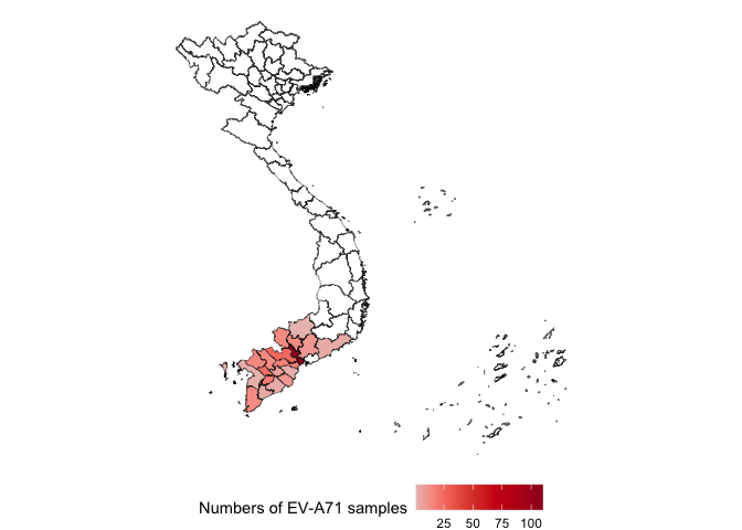
3.2 Time
viro2 <- viro2 %>% filter(city == "tp hcm")

viro_count_p <- viro2 %>%
  mutate(adm_month = as.Date(floor_date(admission_date, "month"))) %>%
  group_by(adm_month,sero_gr) %>%
  count() %>%
  ungroup() %>%
  group_by(adm_month) %>%
  mutate(perc = n / sum(n)) %>%
  ungroup


viro_count_p %>%
ggplot(aes(x = adm_month,y=n,fill = sero_gr))+
  geom_col()+
  scale_x_date(date_labels = "%b",
               date_breaks = "1 month",
               limits = c(as.Date("2023-05-01"),
                          as.Date("2023-12-01")))+
  labs(fill = "Sero group", y = "Number of samples",x = "Month of admission")+
  theme_minimal()+
  theme(legend.position="bottom")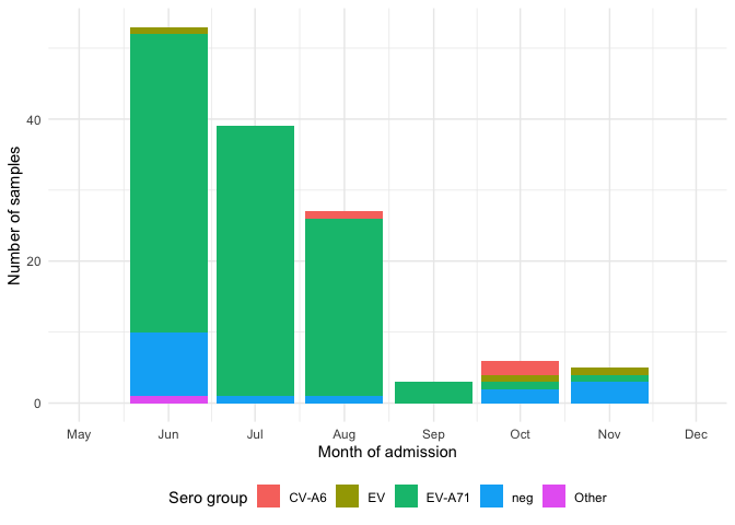
viro_count_p %>% filter(sero_gr == "EV-A71")  %>%
  ggplot(aes(x = adm_month,y=perc))+
  geom_col()+
  scale_x_date(date_labels = "%b",
               date_breaks = "1 month",
               limits = c(as.Date("2023-05-01"),
                          as.Date("2023-12-01")))+
  labs(y = "Percentage of EV-A71 samples",x = "Month of admission")+
  theme_minimal()+
  theme(legend.position="bottom")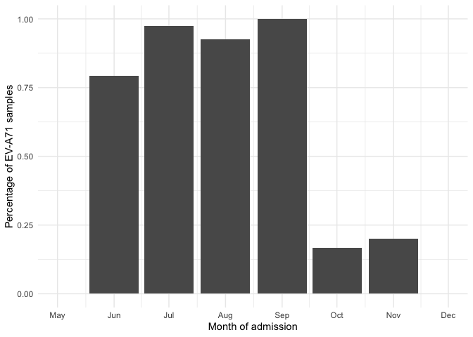
3.3 Epidemiology analysis
3.4 Analyse first peak and the second peak
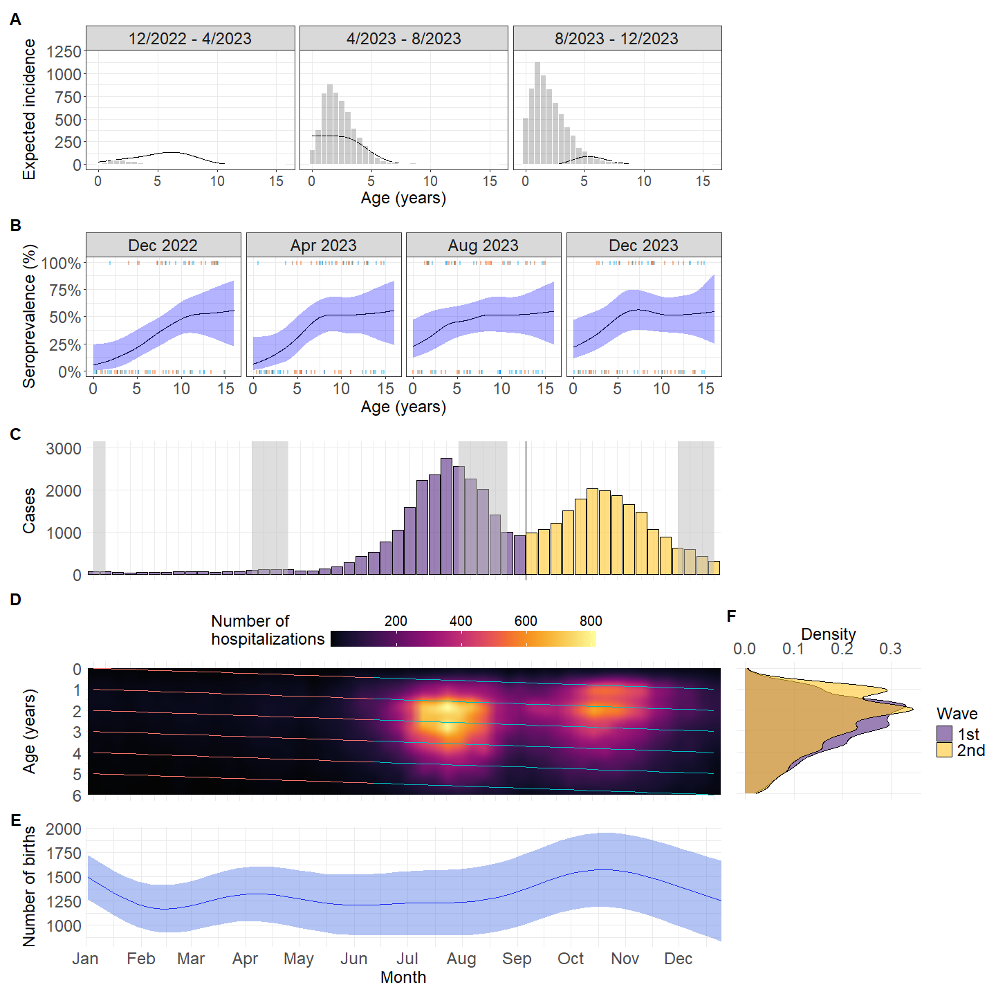
Based on the figure 1, I separate sample from June - Aug as the 1st peak, and from Sep-Dec as the 2nd peak
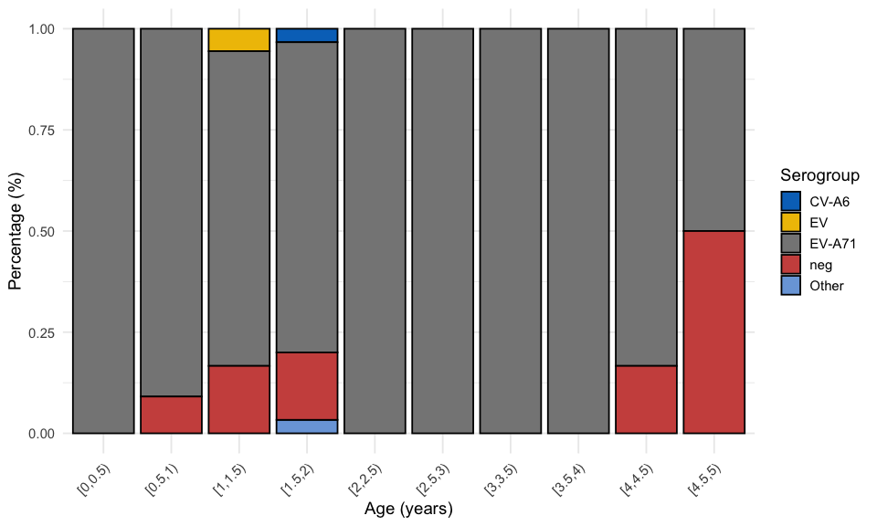
3.4.1 First peak
viro2 %>%
  mutate() %>%
  na.omit() %>%
  filter(month(adm_month2) >= 6 & month(adm_month2) <= 8) %>%
  na.omit() %>%
  group_by(age_bin, sero_gr) %>%
  summarise(n = n(), .groups = "drop_last") %>%
  mutate(perc = n / sum(n)) %>%
  ungroup() %>%
  ggplot(aes(x = age_bin, y = perc, fill = sero_gr)) +
  geom_col(position = "stack", color = "black") +
  ggsci::scale_fill_jco() +
  labs(x = "Age (years)", y = "Percentage (%)", fill = "Serogroup") +
  theme_minimal(base_size = 14) +
  theme(
    axis.text.x = element_text(angle = 45, hjust = 1)
  )
viro2 %>%
  mutate() %>%
  na.omit() %>%
  filter(month(adm_month2) >= 6 & month(adm_month2) <= 8) %>%
  na.omit() %>%
  filter(sero_gr == "EV-A71") %>%
  ggplot(aes(age_adm)) +
  geom_histogram(binwidth = 0.5,
                 color = "white",fill = "black",alpha = 0.5)+
  labs(x = "Age (years)", y = "Number of EV-A71 samples") +
  theme_minimal()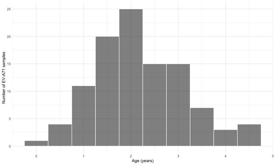
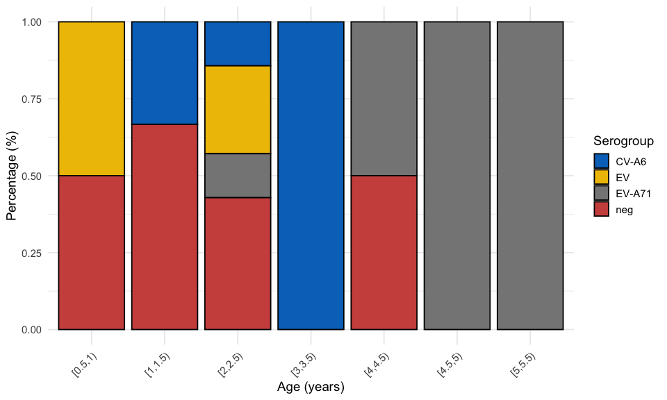
3.4.2 Second peak
viro2 %>%
  mutate() %>%
  na.omit() %>%
  filter(month(adm_month2) >= 9) %>%
  na.omit() %>%
  group_by(age_bin, sero_gr) %>%
  summarise(n = n(), .groups = "drop_last") %>%
  mutate(perc = n / sum(n)) %>%
  ungroup() %>%
  ggplot(aes(x = age_bin, y = perc, fill = sero_gr)) +
  geom_col(position = "stack", color = "black") +
  ggsci::scale_fill_jco() +
  labs(x = "Age (years)", y = "Percentage (%)", fill = "Serogroup") +
  theme_minimal(base_size = 14) +
  theme(
    axis.text.x = element_text(angle = 45, hjust = 1)
  )
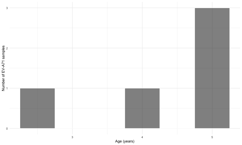
viro2 %>%
  mutate() %>%
  na.omit() %>%
  filter(month(adm_month2) >= 9) %>%
  na.omit() %>%
  filter(sero_gr == "EV-A71") %>%
  ggplot(aes(age_adm)) +
  geom_histogram(binwidth = 0.5,
                 color = "white",fill = "black",alpha = 0.5)+
  labs(x = "Age (years)", y = "Number of EV-A71 samples") +
  theme_minimal()