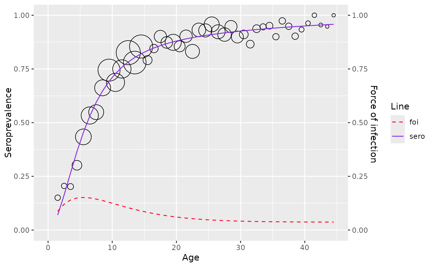
Fit age-stratified seroprevalence data using the Farrington (1990) model, which assumes the force of infection increases linearly with age and subsequently decreases exponentially.
Usage
farrington_model(
  data,
  start,
  fixed = list(),
  age_col = "age",
  pos_col = "pos",
  tot_col = "tot",
  status_col = "status"
)
Arguments
- data
the input data frame, must either have columns for `age`, `pos`, `tot` (for aggregated data) OR `age`, `status` (for linelisting data)
- start
Named list of vectors or single vector. Initial values for optimizer.
- fixed
Named list of vectors or single vector. Parameter values to keep fixed during optimization.
- age_col
name of the `age` column (default age_col="age").
- pos_col
name of the `pos` column (default pos_col="pos").
- tot_col
name of the `tot` column (default tot_col="tot").
- status_col
name of the `status` column (default status_col="status").
Value
a list of class farrington_model with 5 items
- datatype
type of datatype used for model fitting (aggregated or linelisting)
- df
the dataframe used for fitting the model
- info
fitted "mle" object
- sp
seroprevalence
- foi
force of infection
Details
The force of infection is defined as followed
$$ \lambda(a) = (\alpha a - \gamma)e^{-\beta a} + \gamma $$ Where \(\gamma\) is called the long term residual for FOI, as \(a \rightarrow \infty\) , \(\lambda (a) \rightarrow \gamma\)
The seroprevalence can thus be estimated using the non-linear model $$ \pi(a) = 1 - exp\{ \frac{\alpha}{\beta}ae^{-\beta a} + \frac{1}{\beta}(\frac{\alpha}{\beta} - \gamma)(e^{-\beta a} - 1) -\gamma a \} $$
Refer to section 6.1.2. of the the book by Hens et al. (2012) for further details.
References
Hens, Niel, Ziv Shkedy, Marc Aerts, Christel Faes, Pierre Van Damme, and Philippe Beutels. 2012. Modeling Infectious Disease Parameters Based on Serological and Social Contact Data: A Modern Statistical Perspective. tatistics for Biology and Health. Springer New York. doi:10.1007/978-1-4614-4072-7 .
Examples
df <- rubella_uk_1986_1987
model <- farrington_model(
  df,
  start=list(alpha=0.07,beta=0.1,gamma=0.03)
  )
#> Warning: NaNs produced
#> Warning: NaNs produced
#> Warning: NaNs produced
#> Warning: NaNs produced
#> Warning: NaNs produced
#> Warning: NaNs produced
#> Warning: NaNs produced
#> Warning: NaNs produced
#> Warning: NaNs produced
#> Warning: NaNs produced
#> Warning: NaNs produced
#> Warning: NaNs produced
#> Warning: NaNs produced
#> Warning: NaNs produced
#> Warning: NaNs produced
#> Warning: NaNs produced
#> Warning: NaNs produced
#> Warning: NaNs produced
#> Warning: NaNs produced
#> Warning: NaNs produced
#> Warning: NaNs produced
#> Warning: NaNs produced
#> Warning: NaNs produced
#> Warning: NaNs produced
#> Warning: NaNs produced
#> Warning: NaNs produced
#> Warning: NaNs produced
#> Warning: NaNs produced
#> Warning: NaNs produced
#> Warning: NaNs produced
#> Warning: NaNs produced
#> Warning: NaNs produced
#> Warning: NaNs produced
#> Warning: NaNs produced
#> Warning: NaNs produced
#> Warning: NaNs produced
#> Warning: NaNs produced
#> Warning: NaNs produced
#> Warning: NaNs produced
#> Warning: NaNs produced
#> Warning: NaNs produced
#> Warning: NaNs produced
#> Warning: NaNs produced
#> Warning: NaNs produced
#> Warning: NaNs produced
#> Warning: NaNs produced
#> Warning: NaNs produced
#> Warning: NaNs produced
#> Warning: NaNs produced
#> Warning: NaNs produced
#> Warning: NaNs produced
plot(model)
#> Warning: No shared levels found between `names(values)` of the manual scale and the
#> data's fill values.