Penalized splines
Proposed model
A general model relating the prevalence to age can be written as a GLM
\[ g(P(Y_i = 1| a _i)) = g(\pi(a_i)) = \eta(a_i) \]
- Where \(g\) is the link function and \(\eta\) is the linear predictor
The linear predictor can be estimated semi-parametrically using penalized spline with truncated power basis functions of degree \(p\) and fixed knots \(\kappa_1,..., \kappa_k\) as followed
\[ \eta(a_i) = \beta_0 + \beta_1a_i + ... + \beta_p a_i^p + \Sigma_{k=1}^ku_k(a_i - \kappa_k)^p_+ \]
-
Where
\[ (a_i - \kappa_k)^p_+ = \begin{cases} 0, & a_i \le \kappa_k \\ (a_i - \kappa_k)^p, & a_i > \kappa_k \end{cases} \]
In matrix notation, the mean structure model for \(\eta(a_i)\) becomes
\[ \eta = \textbf{X}\beta + \textbf{Zu} \]
Where \(\eta = [\eta(a_i) ... \eta(a_N) ]^T\), \(\beta = [\beta_0 \beta_1 .... \beta_p]^T\), and \(\textbf{u} = [u_1 u_2 ... u_k]^T\) are the regression with corresponding design matrices
\[ \textbf{X} = \begin{bmatrix} 1 & a_1 & a_1^2 & ... & a_1^p \\ 1 & a_2 & a_2^2 & ... & a_2^p \\ \vdots & \vdots & \vdots & \dots & \vdots \\ 1 & a_N & a_N^2 & ... & a_N^p \end{bmatrix}, \textbf{Z} = \begin{bmatrix} (a_1 - \kappa_1 )_+^p & (a_1 - \kappa_2 )_+^p & \dots & (a_1 - \kappa_k)_+^p \\ (a_2 - \kappa_1 )_+^p & (a_2 - \kappa_2 )_+^p & \dots & (a_2 - \kappa_k)_+^p \\ \vdots & \vdots & \dots & \vdots \\ (a_N - \kappa_1 )_+^p & (a_N - \kappa_2 )_+^p & \dots & (a_N - \kappa_k)_+^p \end{bmatrix} \]
FOI can then be derived as
\[ \hat{\lambda}(a_i) = [\hat{\beta_1} , 2\hat{\beta_2}a_i, ..., p \hat{\beta} a_i ^{p-1} + \Sigma^k_{k=1} p \hat{u}_k(a_i - \kappa_k)^{p-1}_+] \delta(\hat{\eta}(a_i)) \]
- Where \(\delta(.)\) is determined by the link function used in the model
Penalized likelihood framework
Proposed approach
The first approach to fit the model is by maximizing the following penalized likelihood
\[\begin{equation} \phi^{-1}[y^T(\textbf{X}\beta + \textbf{Zu} ) - \textbf{1}^Tc(\textbf{X}\beta + \textbf{Zu} )] - \frac{1}{2}\lambda^2 \begin{bmatrix} \beta \\ \textbf{u} \end{bmatrix}^T D\begin{bmatrix} \beta \\ \textbf{u} \end{bmatrix} \tag{1} \end{equation}\]
Where:
\(X\beta + Zu\) is the predictor
\(D\) is a known semi-definite penalty matrix (Wahba 1978), (Green and Silverman 1993)
\(y\) is the response vector
\(\textbf{1}\) is the unit vector, \(c(.)\) is determined by the link function used
\(\lambda\) is the smoothing parameter (larger values –> smoother curves)
\(\phi\) is the overdispersion parameter and equals 1 if there is no overdispersion
Refer to Chapter 8.2.1 of the book by Hens et al. (2012) for a more detailed explanation of the method.
Fitting data
To fit the data using the penalized likelihood framework, specify framework = "pl"
Basis function can be defined via the s parameter, some values for s includes:
"tp"thin plate regression splines"cr"cubic regression splines"ps"P-splines proposed by (Eilers and Marx 1996)"ad"for Adaptive smoothers
For more options, refer to the mgcv documentation (Wood 2017)
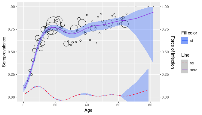
pl <- parvob19_be_2001_2003 %>%
  penalized_spline_model(status_col = "seropositive", s = "tp", framework = "pl")
pl
#> Penalized spline model
#>
#> Input type:  linelisting
#> Framework:  Penalized likelihood
#>
#> Family: binomial
#> Link function: logit
#>
#> Formula:
#> spos ~ s(age, bs = s, sp = sp)
#>
#> Estimated degrees of freedom:
#> 6.16  total = 7.16
#>
#> UBRE score: 0.1206458
plot(pl)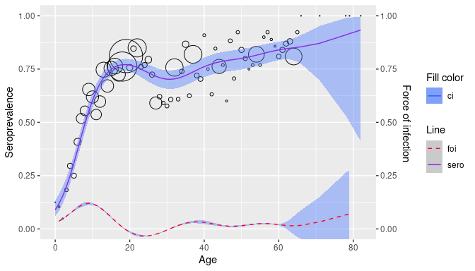
Generalized Linear Mixed Model framework
Proposed approach
Looking back at (1), a constraint for \(\textbf{u}\) would be \(\Sigma_ku_k^2 < C\) for some positive value \(C\)
This is equivalent to choosing \((\beta, \textbf{u})\) to maximise (1) with \(D = diag(\textbf{0}, \textbf{1})\) where \(\textbf{0}\) denotes zero vector length \(p+1\) and \(\textbf{1}\) denotes the unit vector of length \(K\)
For a fixed value for \(\lambda\) this is equivalent to fitting the following generalized linear mixed model Ngo and Wand (2004)
\[ f(y|u) = exp\{ \phi^{-1} [y^T(X\beta + Zu) - c(X\beta + Zu)] + 1^Tc(y)\},\\ u \sim N(0, G) \]
- With similar notations as before and \(G = \sigma^2_uI_{K \times K}\)
Thus \(Z\) is penalized by assuming the corresponding coefficients \(\textbf{u}\) are random effect with \(\textbf{u} \sim N(\textbf{0}, \mathbf{\sigma}^2_u \textbf{I})\).
Refer to Chapter 8.2.2 of the book by Hens et al. (2012) for a more detailed explanation of the method.
Fitting data
To fit the data using the penalized likelihood framework, specify framework = "glmm"
glmm <- parvob19_be_2001_2003 %>%
  penalized_spline_model(status_col = "seropositive", s = "tp", framework = "glmm")
#>
#>  Maximum number of PQL iterations:  20
#> iteration 1
#> iteration 2
#> iteration 3
#> iteration 4
glmm
#> Penalized spline model
#>
#> Input type:  linelisting
#> Framework:  Mixed model
#> $lme
#> Linear mixed-effects model fit by maximum likelihood
#>   Data: data
#>   Log-likelihood: -6977.429
#>   Fixed: fixed
#> X(Intercept)   Xs(age)Fx1
#>    0.7122306    3.6123783
#>
#> Random effects:
#>  Formula: ~Xr - 1 | g
#>  Structure: pdIdnot
#>              Xr1      Xr2      Xr3      Xr4      Xr5      Xr6      Xr7      Xr8
#> StdDev: 6.020273 6.020273 6.020273 6.020273 6.020273 6.020273 6.020273 6.020273
#>         Residual
#> StdDev:        1
#>
#> Variance function:
#>  Structure: fixed weights
#>  Formula: ~invwt
#> Number of Observations: 3080
#> Number of Groups: 1
#>
#> $gam
#>
#> Family: binomial
#> Link function: logit
#>
#> Formula:
#> spos ~ s(age, bs = s, sp = sp)
#>
#> Estimated degrees of freedom:
#> 6.45  total = 7.45
#>
#>
#> attr(,"class")
#> [1] "gamm" "list"
plot(glmm)