library(serosv)
#> Warning: replacing previous import 'magrittr::extract' by 'tidyr::extract' when
#> loading 'serosv'
Imperfect test
Function correct_prevalence() is used for estimating the
true prevalence if the serological test used is imperfect
Arguments:
-
datathe input data frame, must either have:age, pos, tot columns (for aggregated data)
OR age, status columns for (linelisting data)
Users can specifiy the name for these columns in the input data frame using arguments
age_col,pos_col,tot_colorage_col,status_colrespectively
bayesianwhether to adjust sero-prevalence using the Bayesian or frequentist approach. If set toTRUE, true sero-prevalence is estimated using MCMC.init_sesensitivity of the serological test (default value0.95)init_spspecificity of the serological test (default value0.8)study_size_se(applicable whenbayesian=TRUE) sample size for sensitivity validation study (default value1000)study_size_sp(applicable whenbayesian=TRUE) sample size for specificity validation study (default value1000)chains(applicable whenbayesian=TRUE) number of Markov chains (default to1)warmup(applicable whenbayesian=TRUE) number of warm up runs (default value1000)iter(applicable whenbayesian=TRUE) number of iterations (default value2000)
The function will return a list of 2 items:
-
infoif
bayesian = TRUEcontains estimated values for se, sp and corrected seroprevalenceelse return the formula for computing corrected seroprevalence
corrected_seroreturn a data.frame withage,sero(corrected sero) andpos,tot(adjusted based on corrected prevalence)
# ---- estimate real prevalence using Bayesian approach ----
data <- rubella_uk_1986_1987
output <- correct_prevalence(data, warmup = 1000, iter = 4000, init_se=0.9, init_sp = 0.8, study_size_se=1000, study_size_sp=3000)
#>
#> SAMPLING FOR MODEL 'prevalence_correction' NOW (CHAIN 1).
#> Chain 1:
#> Chain 1: Gradient evaluation took 9.4e-05 seconds
#> Chain 1: 1000 transitions using 10 leapfrog steps per transition would take 0.94 seconds.
#> Chain 1: Adjust your expectations accordingly!
#> Chain 1:
#> Chain 1:
#> Chain 1: Iteration:    1 / 4000 [  0%]  (Warmup)
#> Chain 1: Iteration:  400 / 4000 [ 10%]  (Warmup)
#> Chain 1: Iteration:  800 / 4000 [ 20%]  (Warmup)
#> Chain 1: Iteration: 1001 / 4000 [ 25%]  (Sampling)
#> Chain 1: Iteration: 1400 / 4000 [ 35%]  (Sampling)
#> Chain 1: Iteration: 1800 / 4000 [ 45%]  (Sampling)
#> Chain 1: Iteration: 2200 / 4000 [ 55%]  (Sampling)
#> Chain 1: Iteration: 2600 / 4000 [ 65%]  (Sampling)
#> Chain 1: Iteration: 3000 / 4000 [ 75%]  (Sampling)
#> Chain 1: Iteration: 3400 / 4000 [ 85%]  (Sampling)
#> Chain 1: Iteration: 3800 / 4000 [ 95%]  (Sampling)
#> Chain 1: Iteration: 4000 / 4000 [100%]  (Sampling)
#> Chain 1:
#> Chain 1:  Elapsed Time: 2.057 seconds (Warm-up)
#> Chain 1:                4.107 seconds (Sampling)
#> Chain 1:                6.164 seconds (Total)
#> Chain 1:

# check fitted value
output$info[1:2, ]
#>             mean      se_mean          sd      2.5%       25%       50%
#> est_se 0.9278179 0.0001098350 0.006095913 0.9151759 0.9239329 0.9279511
#> est_sp 0.8028005 0.0001011728 0.006973970 0.7888135 0.7981642 0.8028934
#>              75%     97.5%    n_eff      Rhat
#> est_se 0.9318726 0.9390499 3080.323 0.9998417
#> est_sp 0.8075049 0.8167427 4751.518 0.9996668

# ---- estimate real prevalence using frequentist approach ----
freq_output <- correct_prevalence(data, bayesian = FALSE, init_se=0.9, init_sp = 0.8)

# check info
freq_output$info
#> [1] "Formula: real_sero = (observed_sero + sp - 1) / (se + sp -1)"
User can then visualize the output using
plot_corrected_prev() function
# Plot output of the frequentist approach
plot_corrected_prev(freq_output)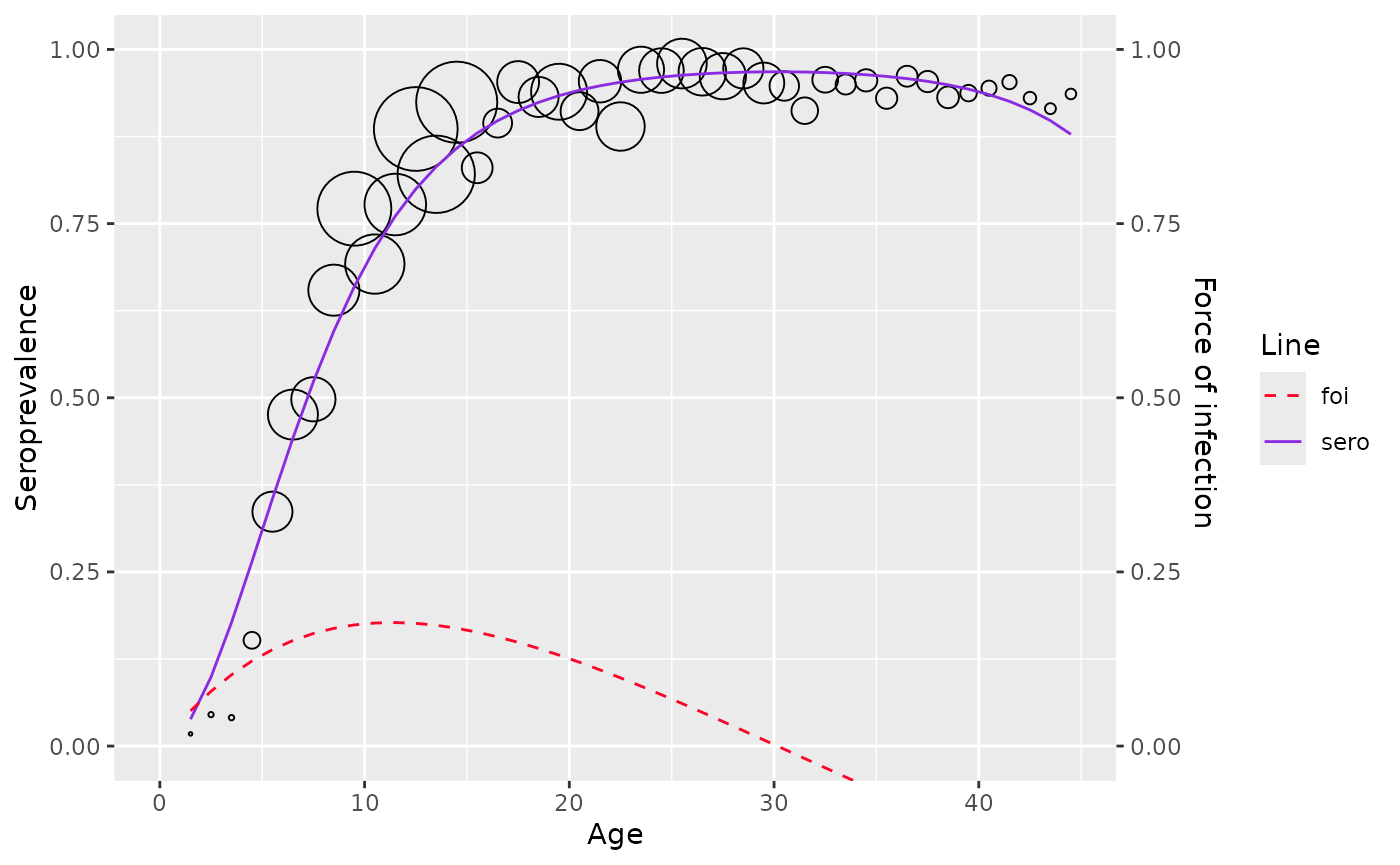
# Plot output of the bayesian approach
plot_corrected_prev(output)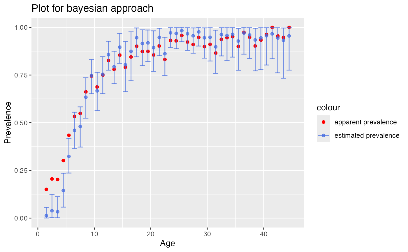
To compare both correction methods in a single plot, provide the
output from the second method as the optional y argument in
plot_corrected_prev()
plot_corrected_prev(output, freq_output)
# set facet = TRUE to display the confidence or credible intervals for each method
plot_corrected_prev(output, freq_output, facet = TRUE)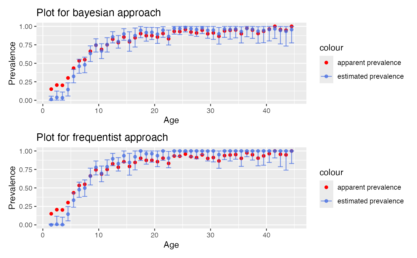
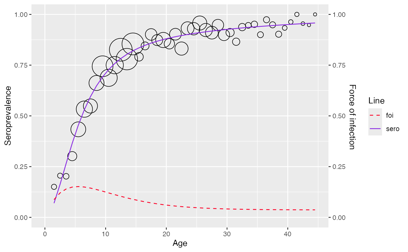
Fitting corrected data
Data after seroprevalence correction
Bayesian approach
suppressWarnings(
  corrected_data <- farrington_model(
  output$corrected_se,
  start=list(alpha=0.07,beta=0.1,gamma=0.03))
)

plot(corrected_data)
#> Warning: No shared levels found between `names(values)` of the manual scale and the
#> data's fill values.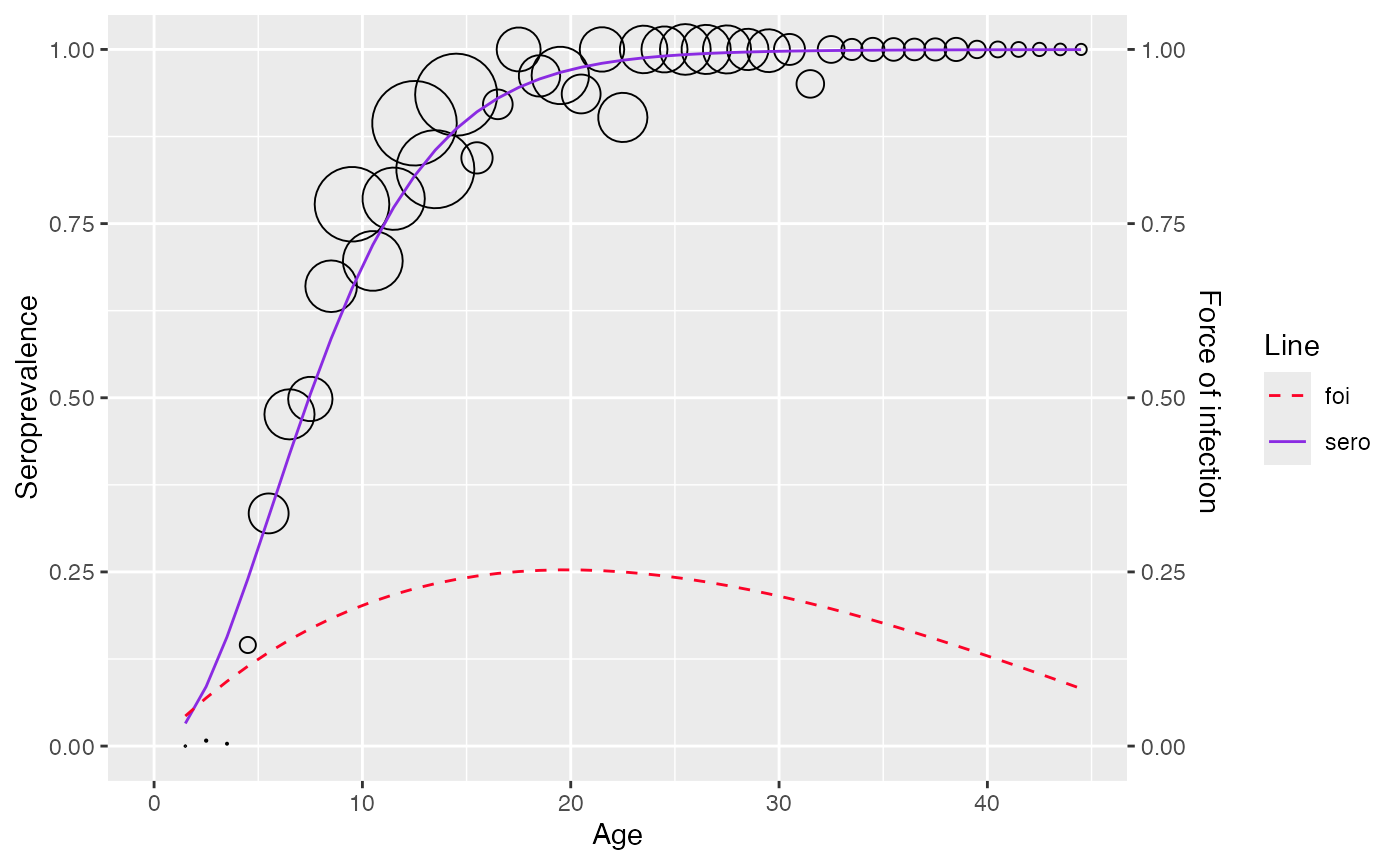
Frequentist approach
suppressWarnings(
  corrected_data <- farrington_model(
  freq_output$corrected_se,
  start=list(alpha=0.07,beta=0.1,gamma=0.03))
)

plot(corrected_data)
#> Warning: No shared levels found between `names(values)` of the manual scale and the
#> data's fill values.
Original data
suppressWarnings(
  original_data <- farrington_model(
  data,
  start=list(alpha=0.07,beta=0.1,gamma=0.03))
)
plot(original_data)
#> Warning: No shared levels found between `names(values)` of the manual scale and the
#> data's fill values.