Model repeated cross-sectional data

library(serosv)
library(dplyr)
library(magrittr)
library(ggplot2)

Age-time varying model

To monitor changes in a population’s seroprevalence over time, modelers often conduct multiple cross-sectional surveys at different time points, each using a new representative sample. The resulting data are known as repeated cross-sectional data.

Proposed approach

To model repeated cross-sectional serological data, serosv offers age_time_model() function which implements the following workflow:

1. Fit age-specific seroprevalence for each survey period
2. Monotonize age-specific or birth-cohort-specific prevalence over time
3. Fit monotonized age-specific seroprevalence for each survey period

Fitting data

The function expects input data with the following columns:

• Either age and status (linelisting) or age and pos + tot (aggregated)

• A column for date of survey (specified via time_col argument)

• A column for id of each survey period (specified via grouping_col argument)

# Prepare data 
tb_nl <- tb_nl_1966_1973 %>% 
  mutate(
    survey_year = age + birthyr,
    survey_time = as.Date(paste0(survey_year, "-01-01"))
  ) %>% select(-birthyr) %>% 
  filter(survey_year > 1966) %>% 
  group_by(age, survey_year, survey_time) %>% 
  summarize(pos = sum(pos), tot = sum(tot), .groups = "drop")

The monotonization method can be specified via the monotonize_method argument, serosv currently supports 2 options:

• Pooled adjacent violators average (monotonize_method = "pava")

• Shape constrained additive model (monotonize_method = "scam")

The users can also configure to monotonize either:

• Age-specific seroprevalence over time (age_correct = FALSE)

• Or birth cohort specific seroprevalence over time (age_correct=TRUE)

out_pava <- tb_nl %>% 
  age_time_model(
    time_col = "survey_time", 
    grouping_col = "survey_year",
    age_correct = F,
    monotonize_method = "pava"
  ) %>% 
  suppressWarnings()

out_scam <- tb_nl %>% 
  age_time_model(
    time_col = "survey_time", 
    grouping_col = "survey_year",
    age_correct = T,
    monotonize_method = "scam"
  ) %>% 
  suppressWarnings()

The output is a data.frame with dimension [number of survey, 9], where each row corresponds to a single survey period. The columns are:

• column for id of survey period

• df - input data.frame corresponding to that survey period

• info - model for the seroprevalence

• monotonized_info - model for the monotonized seroprevalence

• monotonized_ci_mod - model for the monotonized confidence interval

• sp - predicted seroprevalence of the given input data

• foi - estimated force of infection from sp

• monotonized_sp - predicted monotonized seroprevalence of the given input data

• monotonized_foi - estimated force of infection from monotonized_sp

out_pava$out
#> # A tibble: 7 × 9
#>   survey_year monotonized_info monotonized_ci_mod df       info   sp        
#>         <dbl> <list>           <list>             <list>   <list> <list>    
#> 1        1967 <gam>            <named list [2]>   <tibble> <gam>  <dbl [5]> 
#> 2        1968 <gam>            <named list [2]>   <tibble> <gam>  <dbl [5]> 
#> 3        1969 <gam>            <named list [2]>   <tibble> <gam>  <dbl [6]> 
#> 4        1970 <gam>            <named list [2]>   <tibble> <gam>  <dbl [13]>
#> 5        1971 <gam>            <named list [2]>   <tibble> <gam>  <dbl [8]> 
#> 6        1972 <gam>            <named list [2]>   <tibble> <gam>  <dbl [8]> 
#> 7        1973 <gam>            <named list [2]>   <tibble> <gam>  <dbl [5]> 
#> # ℹ 3 more variables: foi <list>, monotonized_sp <list>, monotonized_foi <list>

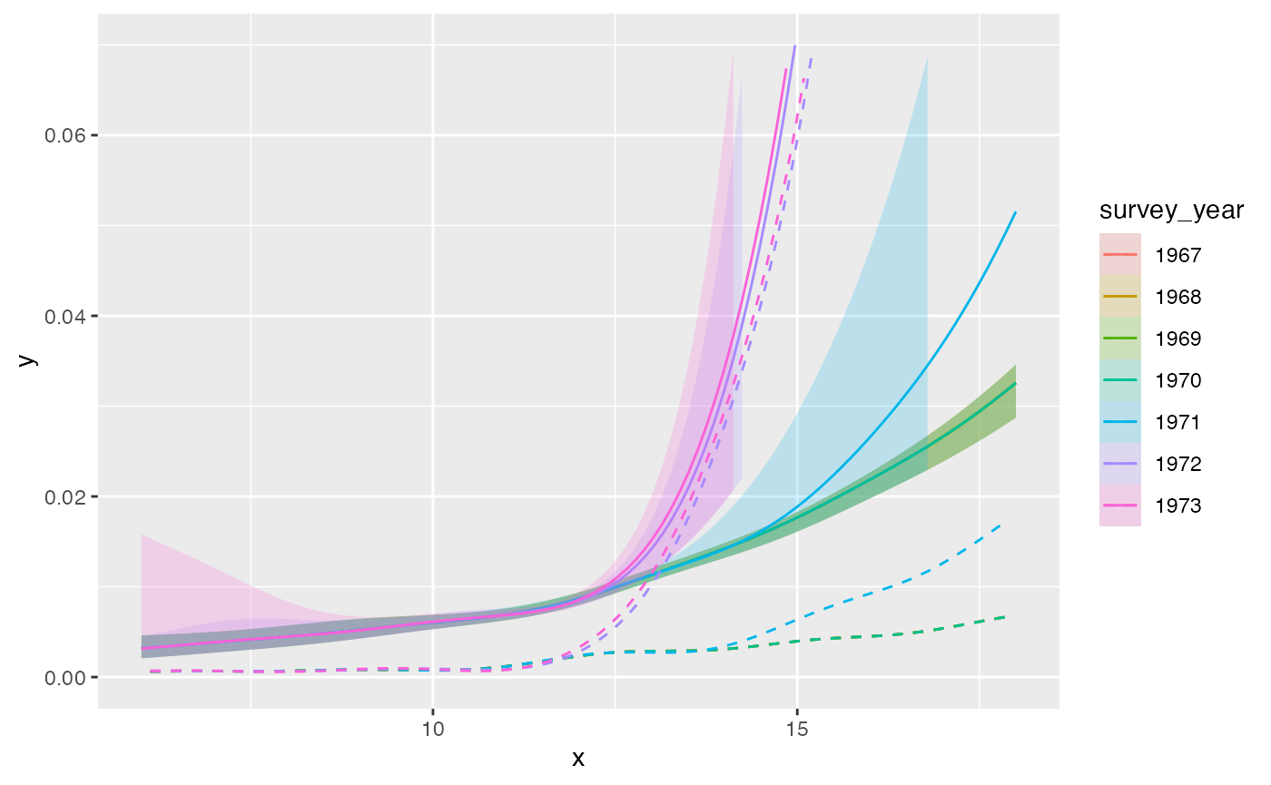
For visualization, the plot function for age_time_model offers the following configurations

• facet whether to visualize result for each survey period separately (facet=TRUE) or on a single plot (facet=FALSE)

• modtype choose which model to visualize, the model fitted with input data (modtype="non-monotonized") or monotonized data (modtype="monotonized")

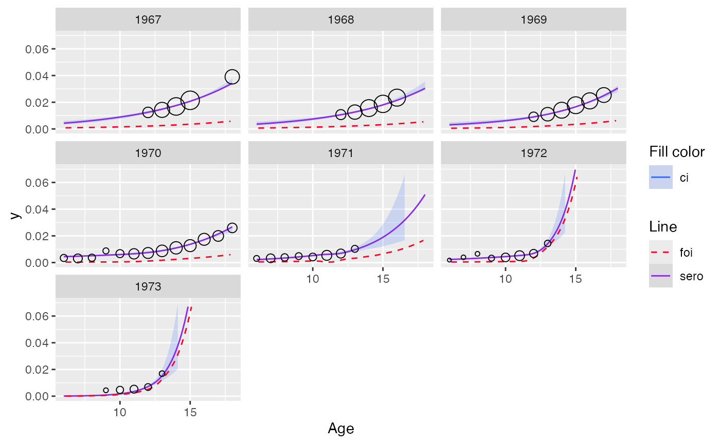
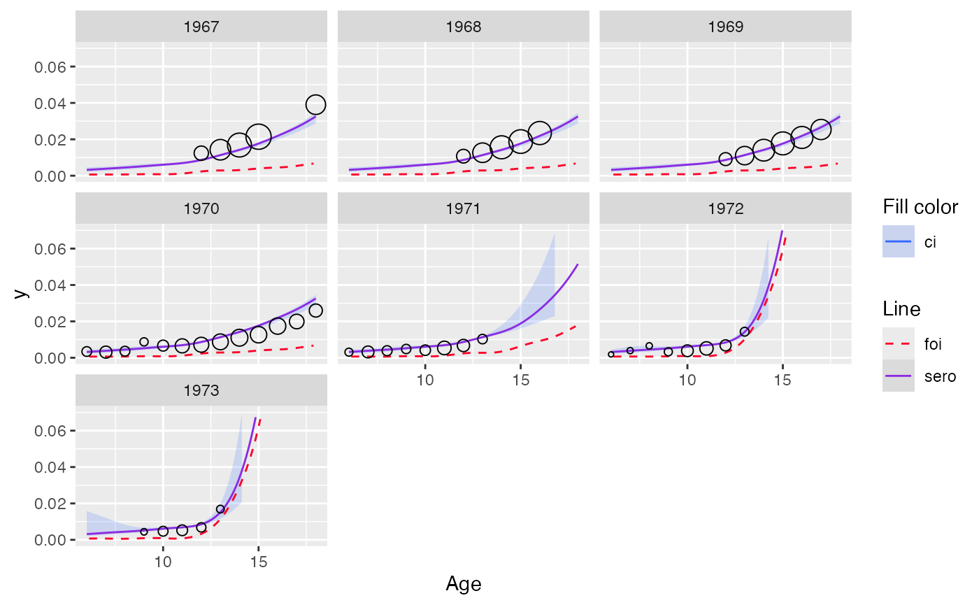
Example: output for model with PAVA for monotonization

plot(out_pava, facet = TRUE, modtype = "non-monotonized") + ylim(c(0, 0.07))
#> Scale for y is already present.
#> Adding another scale for y, which will replace the existing scale.

plot(out_pava, facet = TRUE, modtype = "monotonized") + ylim(c(0, 0.07))
#> Scale for y is already present.
#> Adding another scale for y, which will replace the existing scale.

plot(out_pava, facet = FALSE, modtype = "monotonized") + ylim(c(0, 0.07))
#> Scale for y is already present.
#> Adding another scale for y, which will replace the existing scale.

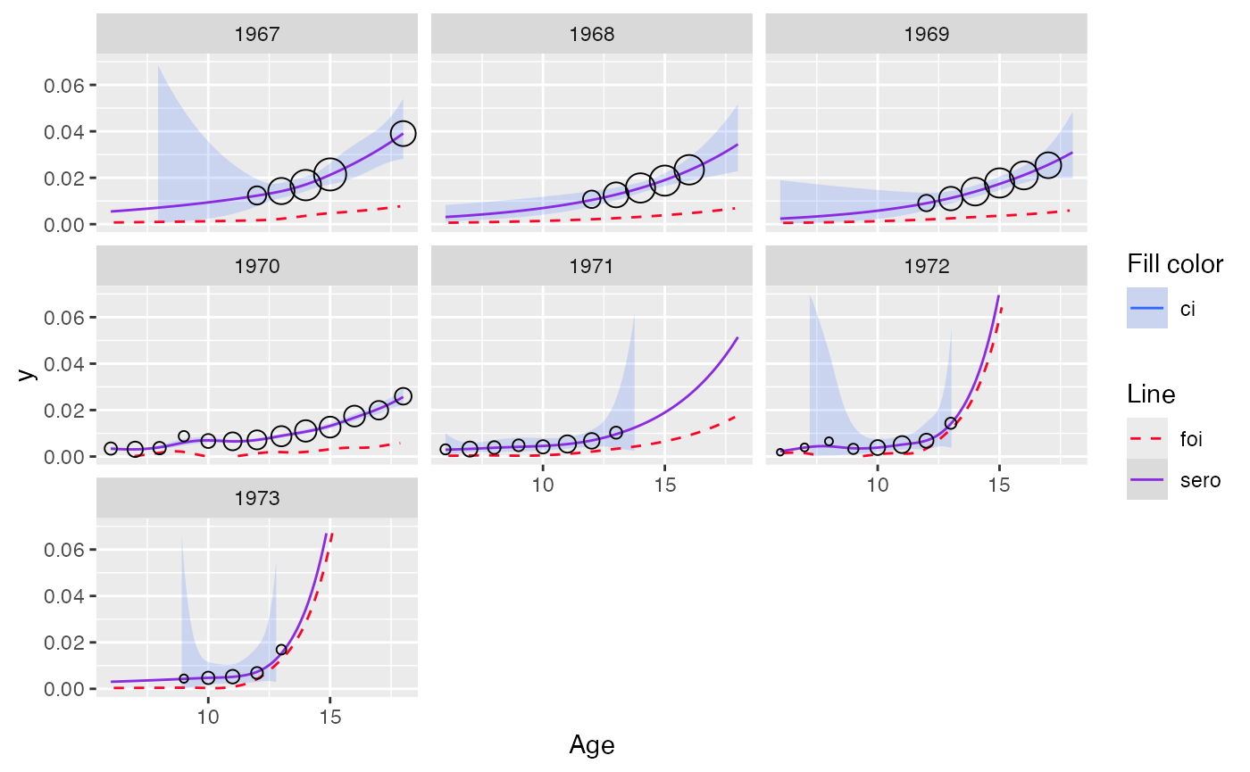
Example: output for model with SCAM for monotonization

plot(out_scam, facet = TRUE, modtype = "non-monotonized") + ylim(c(0, 0.07))
#> Scale for y is already present.
#> Adding another scale for y, which will replace the existing scale.

plot(out_scam, facet = TRUE, modtype = "monotonized") + ylim(c(0, 0.07))
#> Scale for y is already present.
#> Adding another scale for y, which will replace the existing scale.