serosv is an easy-to-use and efficient tool to estimate infectious diseases parameters (seroprevalence and force of infection) using serological data. The current version is mostly based on the book “Modeling Infectious Disease Parameters Based on Serological and Social Contact Data – A Modern Statistical Perspective” by Hens et al., 2012 Springer.
Installation
You can install the development version of serosv with:
# install.packages("devtools")
devtools::install_github("OUCRU-Modelling/serosv")
Feature overview
Datasets
serosv contains 15 built-in serological datasets as provided by Hens et al., 2012 Springer. Simply call the name to load a dataset, for example:
rubella <- rubella_uk_1986_1987Methods
The following methods are available to estimate seroprevalence and force of infection.
Parametric approaches:
-
Frequentist methods:
-
Polynomial models:
- Muench’s model
- Griffiths’ model
- Grenfell and Anderson’s model
-
Nonlinear models:
- Farrington’s model
- Weibull model
Fractional polynomial models
-
-
Bayesian methods:
Hierarchical Farrington model
Hierarchical log-logistic model
Nonparametric approaches:
- Local estimation by polynomials
Semiparametric approaches:
-
Penalized splines:
Penalized likelihood framework
Generalized Linear Mixed Model framework
Demo
Fitting rubella data from the UK
Load the rubella in UK dataset.
Fit the data using a fractional polynomial model via fp_model(). In this example, the model searches for the best combination of powers within a specified range.
rubella_mod <- fp_model(
rubella,
p=list(
p_range=seq(-2,3,0.1), # range of powers to search over
degree=2 # maximum degree for the search
),
monotonic = T, # enforce model to be monotonic
link="logit"
)
rubella_mod
#> Fractional polynomial model
#>
#> Input type: aggregated
#> Powers: -0.9, -0.9
#>
#> Call: glm(formula = as.formula(formulate(curr_p)), family = binomial(link = link))
#>
#> Coefficients:
#> (Intercept) I(age^-0.9)
#> 4.342 -4.696
#> I(I(age^-0.9) * log(age))
#> -9.845
#>
#> Degrees of Freedom: 43 Total (i.e. Null); 41 Residual
#> Null Deviance: 1369
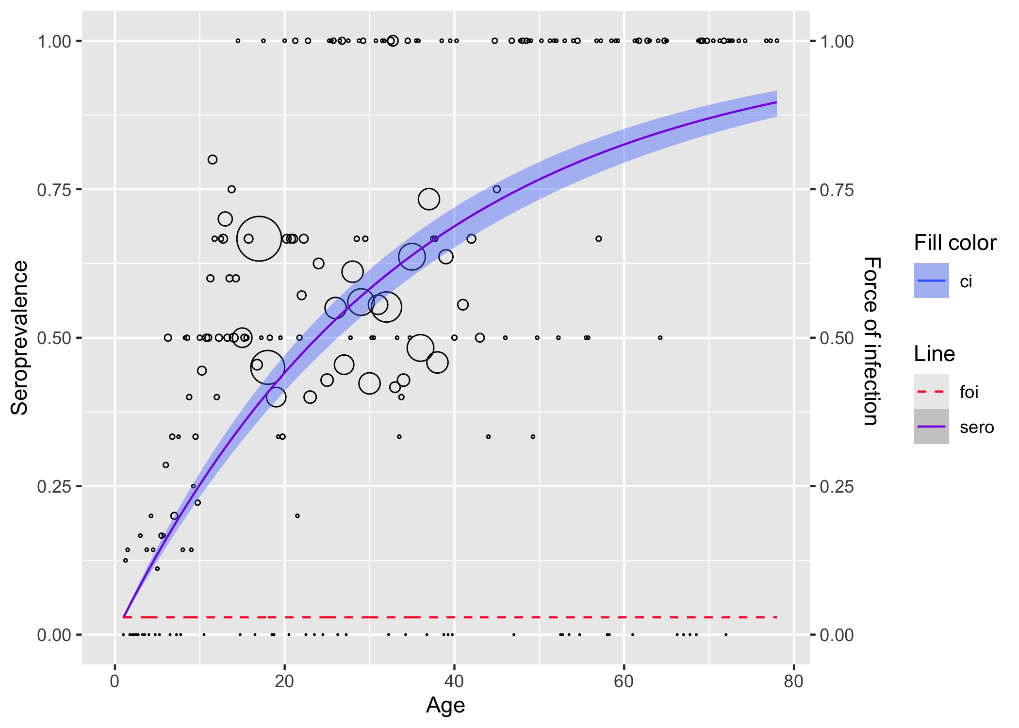
#> Residual Deviance: 37.58 AIC: 210.1Visualize the model
plot(rubella_mod)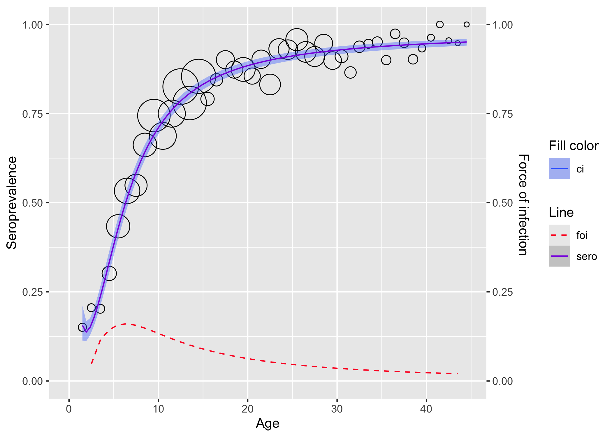
Fitting Parvo B19 data from Finland
library(dplyr)
parvob19 <- parvob19_fi_1997_1998

# for linelisting data, either transform it to aggregated
transform_data(
  parvob19$age,
  parvob19$seropositive,
  stratum_col = "age") |>
  polynomial_model(k = 1) |>
  plot()
# or fit data as is
parvob19 |>
  rename(status = seropositive) |>
  polynomial_model(k = 1) |>
  plot()