Modeling directly from antibody levels • serosv

library(serosv)

Mixture model

Proposed model

Two-component mixture model for test result $Z$ with $Z_j (j = \{I, S\})$ being the latent mixing component having density $f_j(z_j|\theta_j)$ and with $\pi_{\text{TRUE}}(a)$ being the age-dependent mixing probability can be represented as

$f(z|z_I, z_S,a) = (1-\pi_{\text{TRUE}}(a))f_S(z_S|\theta_S)+\pi_{\text{TRUE}}(a)f_I(z_I|\theta_I)$

The mean $E(Z|a)$ thus equals

$\mu(a) = (1-\pi_{\text{TRUE}}(a))\mu_S+\pi_{\text{TRUE}}(a)\mu_I$

From which the true prevalence can be calculated by

$\pi_{\text{TRUE}}(a) = \frac{\mu(a) - \mu_S}{\mu_I - \mu_S}$

Force of infection can then be calculated by

$\lambda_{TRUE} = \frac{\mu'(a)}{\mu_I - \mu(a)}$

Fitting data

To fit the mixture data, use mixture_model function

df <- vzv_be_2001_2003[vzv_be_2001_2003$age < 40.5,]
df <- df[order(df$age),]
data <- df$VZVmIUml
model <- mixture_model(antibody_level = data)
#> Warning in mix(data, starting_values, dist = "norm"): The optimization process
#> terminated because either the estimates are approximate local optimal solution
#> or steptol is too small
model$info
#> 
#> Parameters:
#>       pi    mu  sigma
#> 1 0.1088 2.349 0.6804
#> 2 0.8912 6.439 0.9437
#> 
#> Distribution:
#> [1] "norm"
#> 
#> Constraints:
#>    conpi    conmu consigma 
#>   "NONE"   "NONE"   "NONE"

plot(model)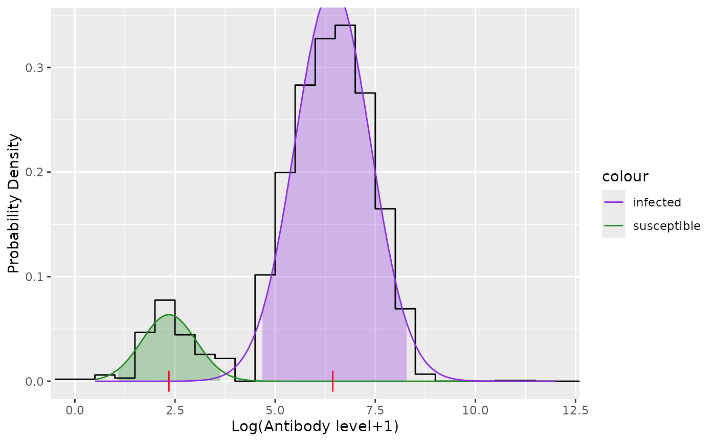

sero-prevalence and FOI can then be esimated using function estimate_from_mixture

est_mixture <- estimate_from_mixture(df$age, data, mixture_model = model, threshold_status = df$seropositive, sp=83, monotonize = FALSE)
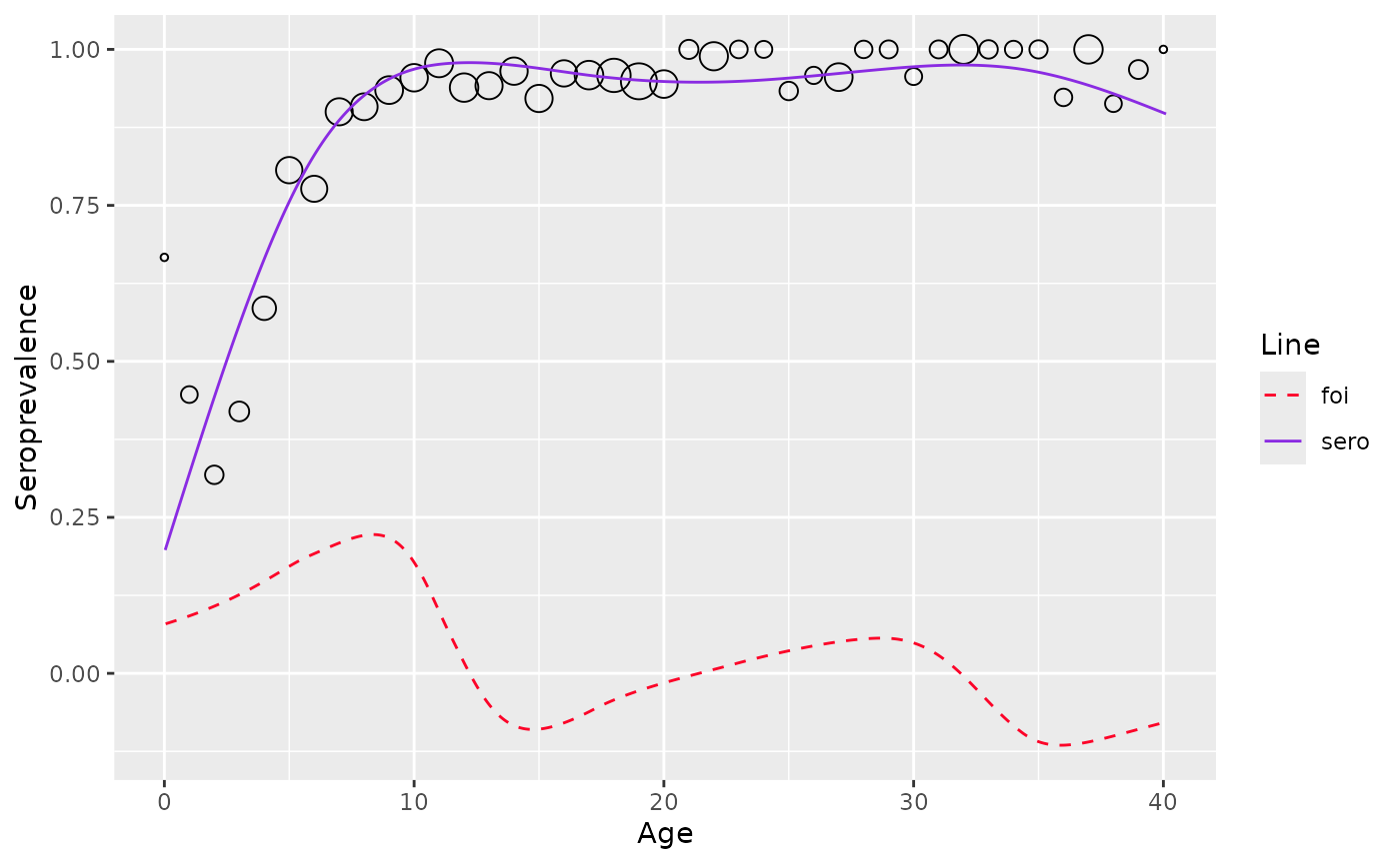
plot(est_mixture)
#> Warning: No shared levels found between `names(values)` of the manual scale and the
#> data's fill values.