Hierarchical Bayesian Model — hierarchical_bayesian

Fit age-stratified seroprevalence to parametric hierarchical Bayesian models. Supported models including Farrington model (2 and 3 parameters variants) and Log Logistic model

Usage

hierarchical_bayesian_model(
  data,
  age_col = "age",
  pos_col = "pos",
  tot_col = "tot",
  status_col = "status",
  type = "far3",
  chains = 1,
  warmup = 1500,
  iter = 5000
)

Arguments

data: the input data frame, must either have columns for `age`, `pos`, `tot` (for aggregated data) OR `age`, `status` (for linelisting data)
age_col: name of the `age` column (default age_col="age").
pos_col: name of the `pos` column (default pos_col="pos").
tot_col: name of the `tot` column (default tot_col="tot").
status_col: name of the `status` column (default status_col="status").
type: type of model ("far2", "far3" or "log_logistic")
chains: number of Markov chains
warmup: number of warmup runs
iter: number of iterations

Value

a list of class hierarchical_bayesian_model with the following items

datatype: type of datatype used for model fitting (aggregated or linelisting)
df: the dataframe used for fitting the model
type: type of bayesian model "far2", "far3" or "log_logistic"
info: a stanfit object for the fitted result
sp: seroprevalence
foi: force of infection
sp_func: function to compute seroprevalence given age and model parameters
foi_func: function to compute force of infection given age and model parameters

Details

Consider a model for prevalence that has a parametric form $\pi(a_i, \alpha)$ where $\alpha$ is a parameter vector

Under a Bayesian framework, we can constraint the parameter space of the prior distribution $P(\alpha)$ to achieve monotonicity of the posterior distribution $P(\pi_1, \pi_2, ..., \pi_m|y,n)$

Where:

- $n = (n_1, n_2, ..., n_m)$ and $n_i$ is the sample size at age $a_i$

- $y = (y_1, y_2, ..., y_m)$ and $y_i$ is the number of infected individual from the $n_i$ sampled subjects

For Farrington model with 3 parameters, prevalence is formulated as follow

$$ \pi (a) = 1 - exp\{ \frac{\alpha_1}{\alpha_2}ae^{-\alpha_2 a} + \frac{1}{\alpha_2}(\frac{\alpha_1}{\alpha_2} - \alpha_3)(e^{-\alpha_2 a} - 1) -\alpha_3 a \} $$

The likelihood model is defined as $y_i \sim Bin(n_i, \pi_i), \text{ for } i = 1,2,3,...m$

The constraint on the parameter space can be incorporated by assuming truncated normal distribution for the components of $\alpha$, $\alpha = (\alpha_1, \alpha_2, \alpha_3)$ in $\pi_i = \pi(a_i,\alpha)$

The flat hyperpriors are defined as $\mu_j \sim \mathcal{N}(0, 10000)$ and $\tau^{-2}_j \sim \Gamma(100,100)$

For Farrington model with 2 parameters, it is equivalent to the previous model with $\alpha_3 = 0$

For Log logistic model, seroprevalence is instead defined as

$$\pi(a) = \frac{\beta a^\alpha}{1 + \beta a^\alpha}, \text{ } \alpha, \beta > 0$$

The likelihood is similarly defined as $y_i \sim Bin(n_i, \pi_i))$

The prior model of $\alpha_1$ is specified as $\alpha_1 \sim \text{truncated } \mathcal{N}(\mu_1, \tau_1)$ with flat hyperpriors as in Farrington model

$\beta$ is constrained to be positive by specifying $\alpha_2 \sim \mathcal{N}(\mu_2, \tau_2)$

Refer to section Chapter 10.3 of the the book by Hens et al. (2012) for further details.

References

Hens, Niel, Ziv Shkedy, Marc Aerts, Christel Faes, Pierre Van Damme, and Philippe Beutels. 2012. Modeling Infectious Disease Parameters Based on Serological and Social Contact Data: A Modern Statistical Perspective. tatistics for Biology and Health. Springer New York. doi:10.1007/978-1-4614-4072-7 .

Examples

# \donttest{
df <- mumps_uk_1986_1987
model <- hierarchical_bayesian_model(df, type="far3")
#> 
#> SAMPLING FOR MODEL 'fra_3' NOW (CHAIN 1).
#> Chain 1: Rejecting initial value:
#> Chain 1:   Log probability evaluates to log(0), i.e. negative infinity.
#> Chain 1:   Stan can't start sampling from this initial value.
#> Chain 1: Rejecting initial value:
#> Chain 1:   Log probability evaluates to log(0), i.e. negative infinity.
#> Chain 1:   Stan can't start sampling from this initial value.
#> Chain 1: 
#> Chain 1: Gradient evaluation took 0.000111 seconds
#> Chain 1: 1000 transitions using 10 leapfrog steps per transition would take 1.11 seconds.
#> Chain 1: Adjust your expectations accordingly!
#> Chain 1: 
#> Chain 1: 
#> Chain 1: Iteration:    1 / 5000 [  0%]  (Warmup)
#> Chain 1: Iteration:  500 / 5000 [ 10%]  (Warmup)
#> Chain 1: Iteration: 1000 / 5000 [ 20%]  (Warmup)
#> Chain 1: Iteration: 1500 / 5000 [ 30%]  (Warmup)
#> Chain 1: Iteration: 1501 / 5000 [ 30%]  (Sampling)
#> Chain 1: Iteration: 2000 / 5000 [ 40%]  (Sampling)
#> Chain 1: Iteration: 2500 / 5000 [ 50%]  (Sampling)
#> Chain 1: Iteration: 3000 / 5000 [ 60%]  (Sampling)
#> Chain 1: Iteration: 3500 / 5000 [ 70%]  (Sampling)
#> Chain 1: Iteration: 4000 / 5000 [ 80%]  (Sampling)
#> Chain 1: Iteration: 4500 / 5000 [ 90%]  (Sampling)
#> Chain 1: Iteration: 5000 / 5000 [100%]  (Sampling)
#> Chain 1: 
#> Chain 1:  Elapsed Time: 17.621 seconds (Warm-up)
#> Chain 1:                10.803 seconds (Sampling)
#> Chain 1:                28.424 seconds (Total)
#> Chain 1: 
#> Warning: There were 790 divergent transitions after warmup. See
#> https://mc-stan.org/misc/warnings.html#divergent-transitions-after-warmup
#> to find out why this is a problem and how to eliminate them.
#> Warning: Examine the pairs() plot to diagnose sampling problems
#> Warning: Bulk Effective Samples Size (ESS) is too low, indicating posterior means and medians may be unreliable.
#> Running the chains for more iterations may help. See
#> https://mc-stan.org/misc/warnings.html#bulk-ess
#> Warning: Tail Effective Samples Size (ESS) is too low, indicating posterior variances and tail quantiles may be unreliable.
#> Running the chains for more iterations may help. See
#> https://mc-stan.org/misc/warnings.html#tail-ess
model$info
#> Inference for Stan model: fra_3.
#> 1 chains, each with iter=5000; warmup=1500; thin=1; 
#> post-warmup draws per chain=3500, total post-warmup draws=3500.
#> 
#>                  mean se_mean      sd     2.5%      25%      50%      75%
#> alpha1           0.14    0.00    0.01     0.13     0.13     0.14     0.14
#> alpha2           0.20    0.00    0.01     0.18     0.19     0.20     0.20
#> alpha3           0.01    0.00    0.01     0.00     0.00     0.01     0.01
#> tau_alpha1       0.06    0.01    0.14     0.00     0.00     0.00     0.03
#> tau_alpha2       0.57    0.18    1.16     0.00     0.00     0.04     0.48
#> tau_alpha3       0.16    0.05    0.37     0.00     0.00     0.01     0.10
#> mu_alpha1        0.60    2.16   44.78   -96.97   -11.21     0.07    12.31
#> mu_alpha2       -0.23    1.75   28.44   -60.60    -2.53     0.28     3.26
#> mu_alpha3        4.83    3.07   45.34   -94.43    -4.41     0.46    12.48
#> sigma_alpha1    96.57   17.94  345.42     1.34     5.42    18.80    58.05
#> sigma_alpha2    53.34   10.72  383.00     0.49     1.44     5.24    24.32
#> sigma_alpha3   136.93   49.26 1201.90     0.90     3.19    14.13    51.62
#> lp__         -2535.56    0.29    3.56 -2542.88 -2538.01 -2535.34 -2532.97
#>                 97.5% n_eff Rhat
#> alpha1           0.15    43 1.04
#> alpha2           0.22    41 1.02
#> alpha3           0.02   245 1.00
#> tau_alpha1       0.56   197 1.00
#> tau_alpha2       4.23    42 1.00
#> tau_alpha3       1.23    47 1.00
#> mu_alpha1      109.84   431 1.02
#> mu_alpha2       57.56   263 1.00
#> mu_alpha3      107.19   218 1.00
#> sigma_alpha1   676.53   371 1.00
#> sigma_alpha2   324.42  1276 1.00
#> sigma_alpha3   791.76   595 1.00
#> lp__         -2529.63   149 1.01
#> 
#> Samples were drawn using NUTS(diag_e) at Tue Jul 28 14:55:01 2026.
#> For each parameter, n_eff is a crude measure of effective sample size,
#> and Rhat is the potential scale reduction factor on split chains (at 
#> convergence, Rhat=1).
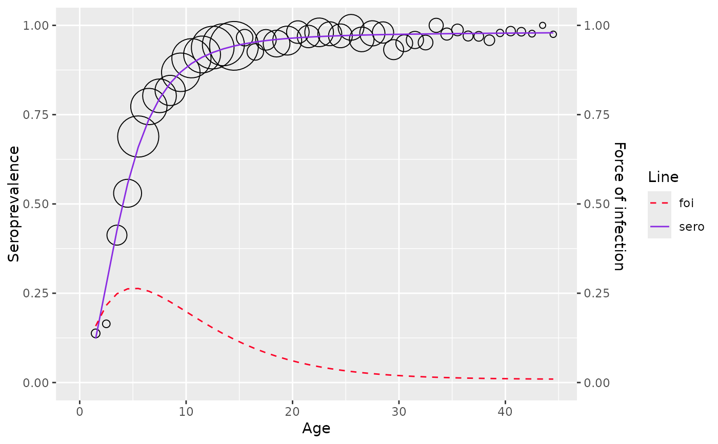
plot(model)

# }