SIR model • serosv

library(serosv)

Basic SIR model

Proposed model

A transmission model consists of 3 compartments: susceptible (S), infected (I), recovered (R)

With the following assumptions:

Individuals are born into susceptible group (exposure time is age of the individual) then transfer to infected class and recovered class
Recovered individuals gained lifelong immunity
Age homogeneity

And described by a system of 3 differential equations

$\begin{cases} \frac{dS(t)}{dt} = B(t) (1-p) - \lambda(t)S(t) - \mu S(t) \\ \frac{dI(t)}{dt} = \lambda(t)S(t) - \nu I(t) - \mu I(t) - \alpha I(t) \\ \frac{dR(t)}{dt} = B(t) p + \nu I(t) - \mu R(t) \end{cases}$

Where:

$B(t) = \mu N(t)$
$\lambda(t) = \beta I(t)$ with $\beta$ is the transmission rate
$\mu$ is the natural death rate
$\nu$ is the recovery rate
$\alpha$ is the disease related death rate
$p$ is the proportion of newborn vaccinated and moved directly to the recovered compartment

Fitting data

To fit a basic SIR model, use sir_basic_model() and specify the following parameters

state - initial population of each compartment
times - a time sequence
parameters - parameters for SIR model

state <- c(S=4999, I=1, R=0)
parameters <- c(
  mu=1/75, # 1 divided by life expectancy (75 years old)
  alpha=0, # no disease-related death
  beta=0.0005, # transmission rate
  nu=1, # 1 year for infected to recover
  p=0 # no vaccination at birth
)
times <- seq(0, 250, by=0.1)
model <- sir_basic_model(times, state, parameters)
model$parameters
#>         mu      alpha       beta         nu          p 
#> 0.01333333 0.00000000 0.00050000 1.00000000 0.00000000
plot(model)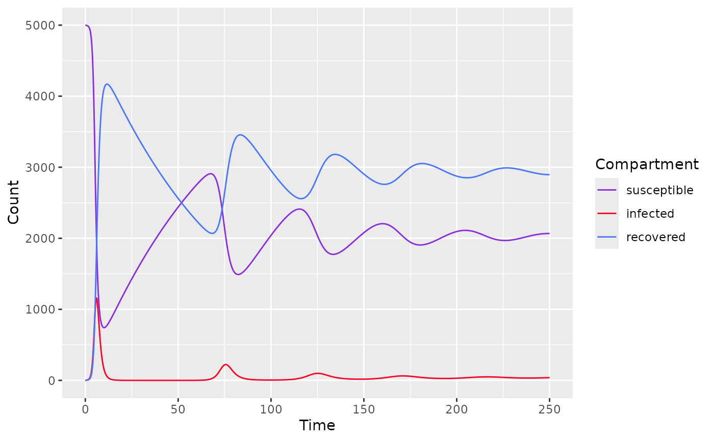

SIR model with constant Force of Infection at Endemic state

Proposed model

A transmission model consists of 3 compartments: susceptible (S), infected (I), recovered (R)

With the following assumptions:

Time homogeneity
Age heterogeneity

Described by a system of 3 differential equations

$\begin{cases} \frac{ds(a)}{da} = -\lambda s(a) \\ \frac{di(a)}{da} = \lambda s(a) - \nu i(a) \\ \frac{dr(a)}{da} = \nu i(a) \end{cases}$

Where:

$s(a), i(a), r(a)$ are proportion of susceptible, infected, recovered population of age group $a$ respectively
$\lambda$ is the force of infection
$\nu$ is the recovery rate

FItting data

To fit an SIR model with constant FOI, use sir_static_model() and specify the following parameters

state - initial proportion of each compartment
ages - an age sequence
parameters - parameters for the model

state <- c(s=0.99,i=0.01,r=0)
parameters <- c(
  lambda = 0.05,
  nu=1/(14/365) # 2 weeks to recover
)
ages<-seq(0, 90, by=0.01)
model <- sir_static_model(ages, state, parameters)
model$parameters
#>   lambda       nu 
#>  0.05000 26.07143
plot(model)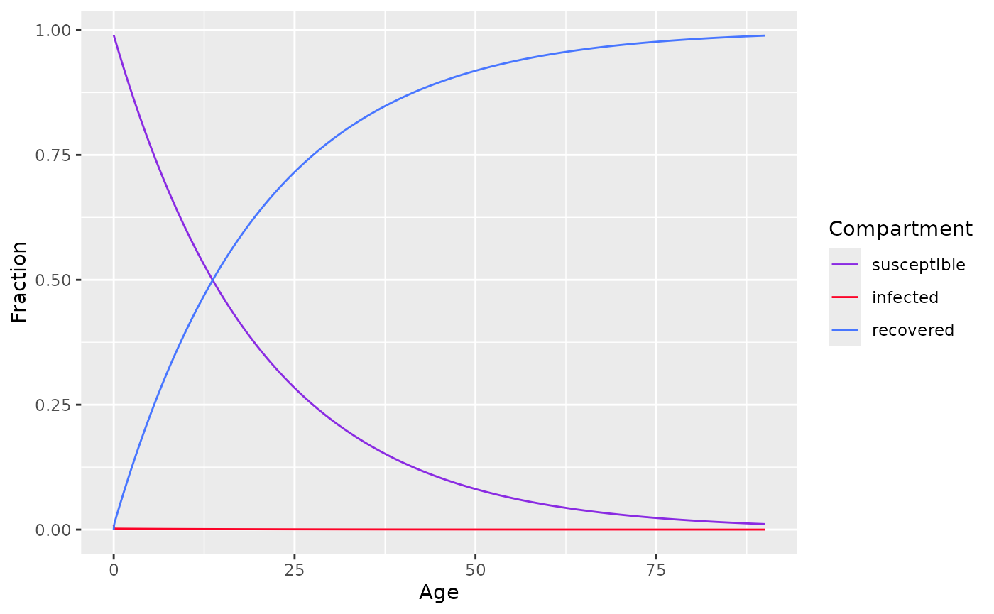

SIR model with sub populations

Proposed model

Extends on the SIR model by having interacting sub-populations (different age groups)

With K subpopulations, the WAIFW matrix or mixing matrix is given by

$C = \begin{bmatrix} \beta_{11} & \beta_{12} & ... & \beta_{1K} \\ \beta_{21} & \beta_{22} & ... & \beta_{2K} \\ \vdots & \vdots & ... & \vdots \\ \beta_{K1} & \beta_{K2} & ... & \beta_{KK} \\ \end{bmatrix}$

The system of differential equations for the i $th$ subpopulation is given by

$\begin{cases} \frac{dS_i(t)}{dt} = -(\sum^K_{j=1}\beta_{ij}I_j(t)) S_i(t) + N_i\mu_i - \mu_i S_i(t) \\ \frac{dI_i(t)}{dt} = (\sum^K_{j=1}\beta_{ij}I_j(t)) S_i(t) - (\nu_i + \mu_i) I_i(t) \\ \frac{dR_i(t)}{dt} = \nu_i I_i(t) - \mu_i R_i(t) \end{cases}$

FItting data

To fit a SIR model with subpopulations, use sir_subpops_model() and specify the following parameters

state - initial proportion of each compartment for each population
beta_matrix - the WAIFW matrix
times - a time sequence
parameters - parameters for the model

k <- 2 # number of population
state <- c(
  # proportion of each compartment for each population
  s = c(0.8, 0.6), 
  i = c(0.2, 0.4),
  r = c(  0,   0)
)
beta_matrix <- c(
  c(0.05, 0.00),
  c(0.00, 0.05)
)
parameters <- list(
  beta = matrix(beta_matrix, nrow=k, ncol=k, byrow=TRUE),
  nu = c(1/30, 1/30),
  mu = 0.001,
  k = k
)
times<-seq(0,10000,by=0.5)
model <- sir_subpops_model(times, state, parameters)
model$parameters
#> $beta
#>      [,1] [,2]
#> [1,] 0.05 0.00
#> [2,] 0.00 0.05
#> 
#> $nu
#> [1] 0.03333333 0.03333333
#> 
#> $mu
#> [1] 0.001
#> 
#> $k
#> [1] 2
plot(model) # returns plot for each population
#> $subpop_1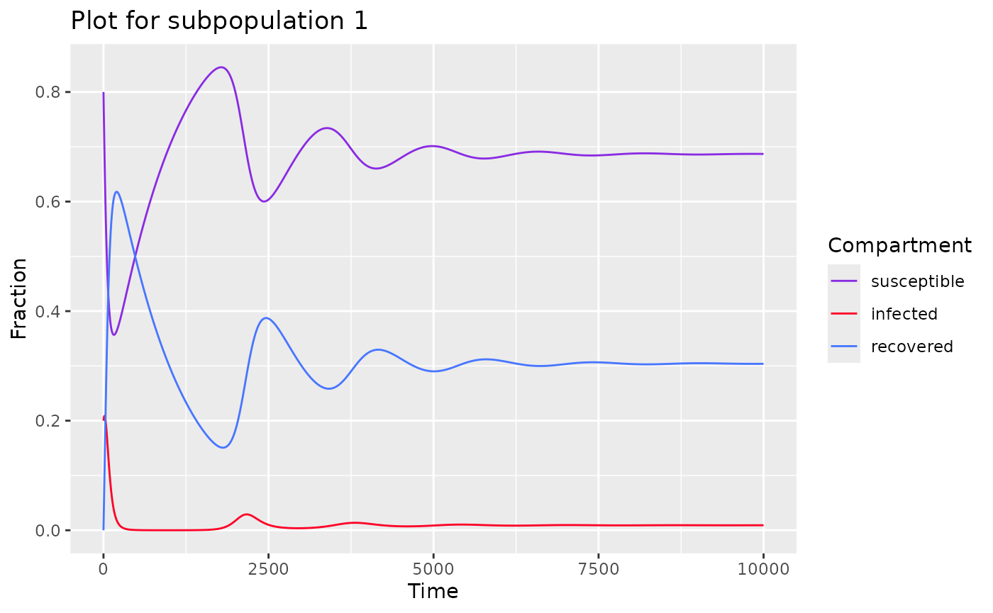

#> 
#> $subpop_2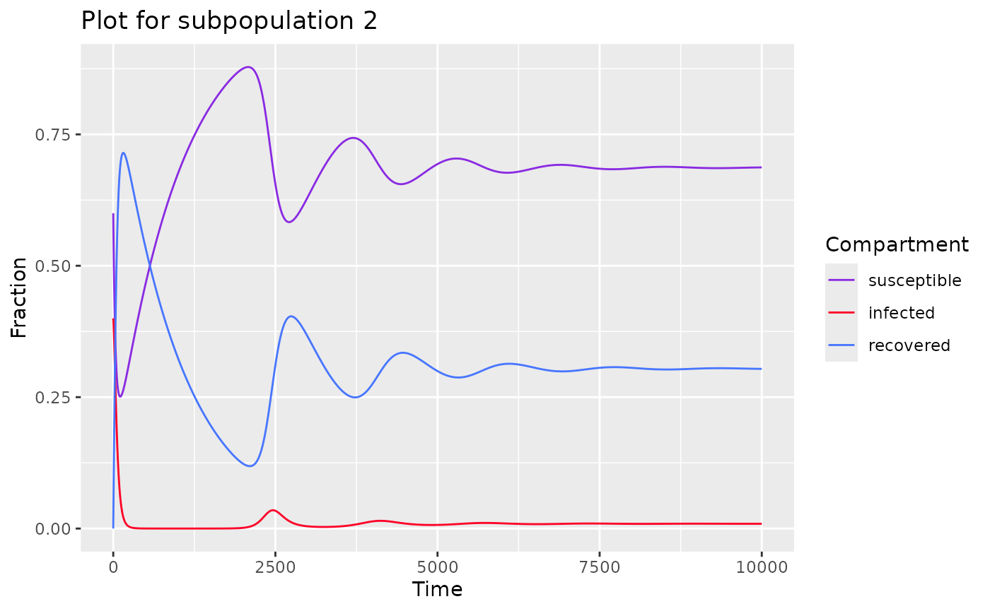

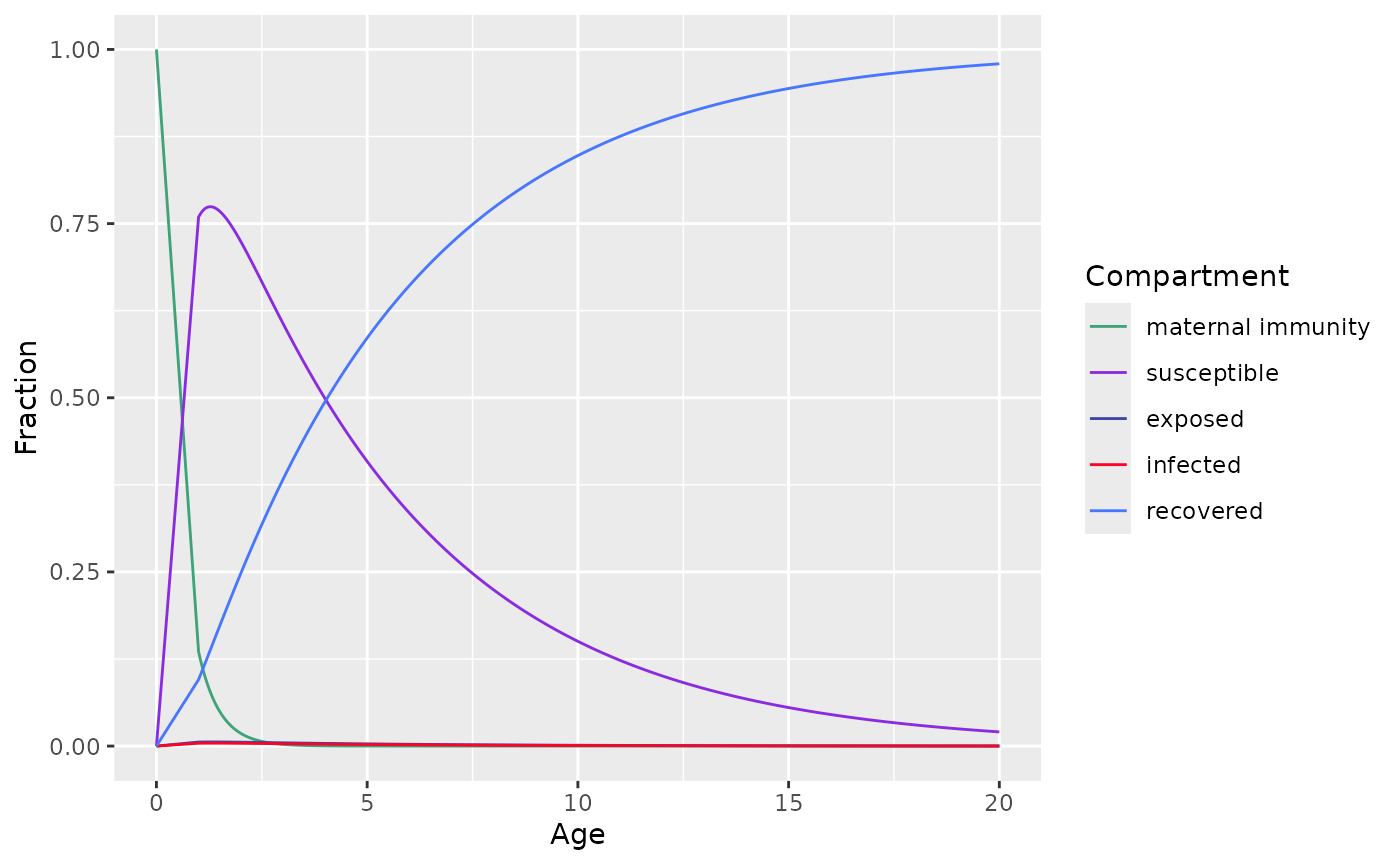
MSEIR model

Proposed model

Extends on SIR model with 2 additional compartments: maternal antibody (M) and exposed period (E)

And described by the following system of ordinary differential equation

$\begin{cases} \frac{dM(a)}{da} = -(\gamma + \mu(a))M(a) \\ \frac{dS(a)}{da} = \gamma M(a) - (\lambda(a) + \mu(a)) S(a) \\ \frac{dE(a)}{da} = \lambda(a) S(a) - (\sigma + \mu(a)) E(a) \\ \frac{dI(a)}{da} = \sigma(a) E(a) - (\nu + \mu(a)) I(a) \\ \frac{dR(a)}{da} = \nu I(a) - \mu(a) R(a) \end{cases}$

Where

$M(0)$ = B, the number of births in the population
$\gamma$ is the rate of antibody decaying
$\lambda(a)$ is the force of infection at age $a$
$\mu(a)$ is the natural death rate at age $a$
$\sigma$ is the rate of becoming infected after being exposed
$\nu$ is the recovery rate

Fitting data

To fit a MSEIR, use mseir_model() and specify the following parameters

a - age sequence
And model parameters including gamma, lambda, sigma, nu

model <- mseir_model(
  a=seq(from=1,to=20,length=500), # age range from 0 -> 20 yo
  gamma=1/0.5, # 6 months in the maternal antibodies
  lambda=0.2,  # 5 years in the susceptible class
  sigma=26.07, # 14 days in the latent class
  nu=36.5      # 10 days in the infected class
)
model$parameters
#> $gamma
#> [1] 2
#> 
#> $lambda
#> [1] 0.2
#> 
#> $sigma
#> [1] 26.07
#> 
#> $nu
#> [1] 36.5
plot(model)

Hens, Niel, Ziv Shkedy, Marc Aerts, Christel Faes, Pierre Van Damme, and Philippe Beutels. 2012. Modeling Infectious Disease Parameters Based on Serological and Social Contact Data: A Modern Statistical Perspective. Statistics for Biology and Health. Springer New York. https://doi.org/10.1007/978-1-4614-4072-7.