Penalized Spline model

Fit age-specific seroprevalence to a semi-parametric model where predictor is modeled with penalized splines. The penalized splines can be estimated by either (1) penalized likelihood framework or (2) mixed model framework

Usage

penalized_spline_model(
  data,
  age_col = "age",
  pos_col = "pos",
  tot_col = "tot",
  status_col = "status",
  s = "bs",
  link = "logit",
  framework = "pl",
  sp = NULL
)

Arguments

data: the input data frame, must either have columns for `age`, `pos`, `tot` (for aggregated data) OR columns for `age`, `status` (for linelisting data)
age_col: name of the `age` column (default age_col="age").
pos_col: name of the `pos` column (default pos_col="pos").
tot_col: name of the `tot` column (default tot_col="tot").
status_col: name of the `status` column (default status_col="status").
s: smoothing basis to use
link: link function to use
framework: which approach to fit the model ("pl" for penalized likelihood framework, "glmm" for generalized linear mixed model framework)
sp: smoothing parameter

Value

a list of class penalized_spline_model with 6 attributes

datatype: type of datatype used for model fitting (aggregated or linelisting)
df: the dataframe used for fitting the model
framework: either pl or glmm
info: fitted "gam" model when framework is pl or "gamm" model when framework is glmm
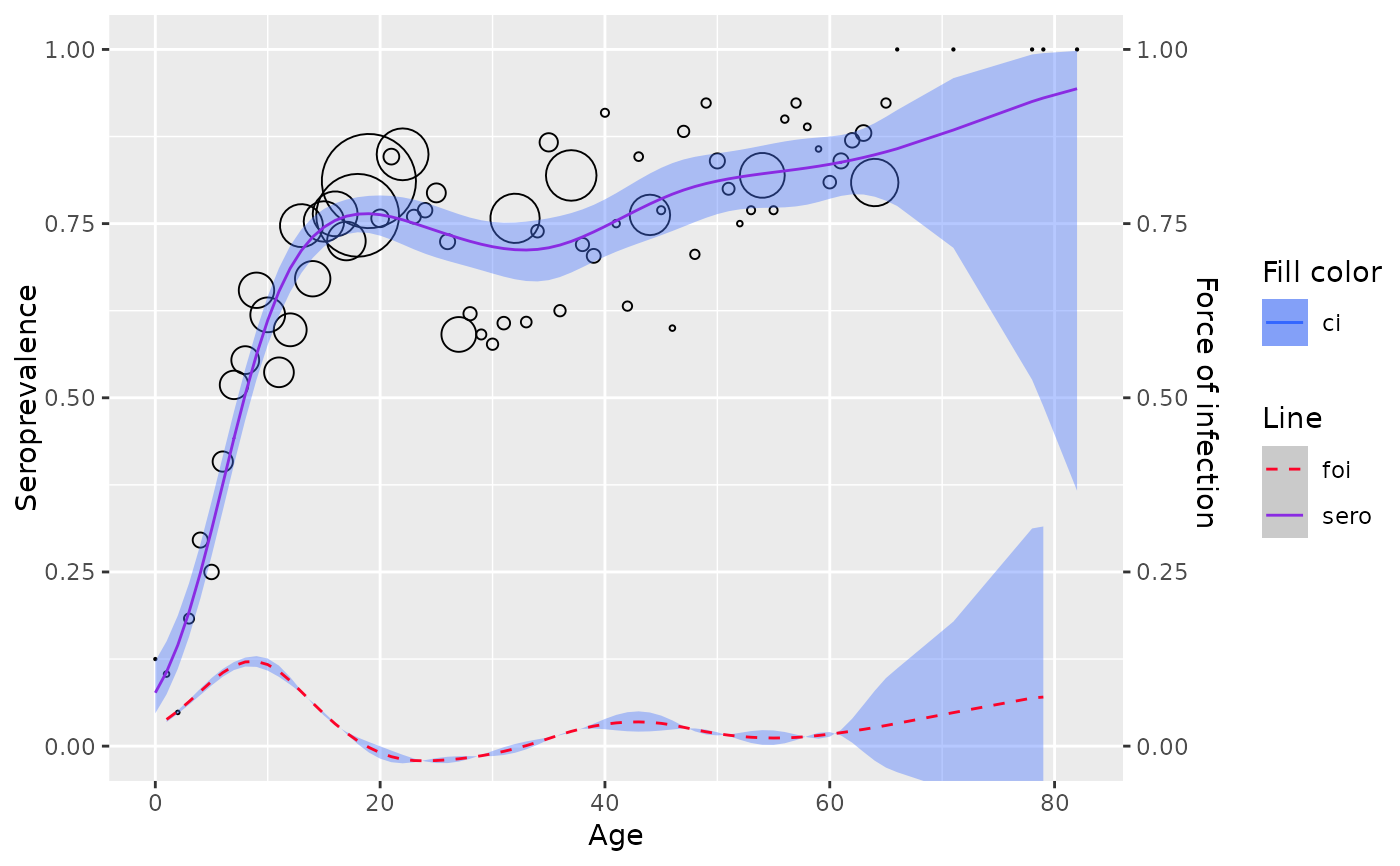
sp: seroprevalence
foi: force of infection

Details

In the semi-parametric model, the predictor is formulated as a penalized spline with truncated power basis functions of degree $p$ and fixed knots $\kappa_1,..., \kappa_k$ as followed

$$ \eta(a_i) = \beta_0 + \beta_1a_i + ... + \beta_p a_i^p + \Sigma_{k=1}^ku_k(a_i - \kappa_k)^p_+ $$

- Where: $$ (a_i - \kappa_k)^p_+ = \begin{cases} 0, & a_i \le \kappa_k \\ (a_i - \kappa_k)^p, & a_i > \kappa_k \end{cases} $$

FOI can then be derived by

$$\hat{\lambda}(a_i) = [\hat{\beta_1} , 2\hat{\beta_2}a_i, ..., p \hat{\beta} a_i ^{p-1} + \Sigma^k_{k=1} p \hat{u}_k(a_i - \kappa_k)^{p-1}_+] \delta(\hat{\eta}(a_i)) $$

Where $\delta(.)$ is determined by the link function used in the model

In matrix annotation, the mean structure model for $\eta(a_i)$ becomes $$\eta = \textbf{X}\beta + \textbf{Zu}$$

Where $\eta = [\eta(a_i) ... \eta(a_N) ]^T$, $\beta = [\beta_0 \beta_1 .... \beta_p]^T$, and $\textbf{u} = [u_1 u_2 ... u_k]^T$ are the regression with corresponding design matrices $$\textbf{X} = \begin{bmatrix} 1 & a_1 & a_1^2 & ... & a_1^p \\ 1 & a_2 & a_2^2 & ... & a_2^p \\ \vdots & \vdots & \vdots & \dots & \vdots \\ 1 & a_N & a_N^2 & ... & a_N^p \end{bmatrix}, \textbf{Z} = \begin{bmatrix} (a_1 - \kappa_1 )_+^p & (a_1 - \kappa_2 )_+^p & \dots & (a_1 - \kappa_k)_+^p \\ (a_2 - \kappa_1 )_+^p & (a_2 - \kappa_2 )_+^p & \dots & (a_2 - \kappa_k)_+^p \\ \vdots & \vdots & \dots & \vdots \\ (a_N - \kappa_1 )_+^p & (a_N - \kappa_2 )_+^p & \dots & (a_N - \kappa_k)_+^p \end{bmatrix} $$

Under penalized likelihood framework, the model is fitted by maximizing the following likelihood

$$ \phi^{-1}[y^T(\textbf{X}\beta + \textbf{Zu} ) - \textbf{1}^Tc(\textbf{X}\beta + \textbf{Zu} )] - \frac{1}{2}\lambda^2 \begin{bmatrix} \beta \\ \textbf{u} \end{bmatrix}^T D\begin{bmatrix} \beta \\ \textbf{u} \end{bmatrix} $$

Where:

- $X\beta + Zu$ is the predictor

- $D$ is a known semi-definite penalty matrix [@Wahba1978], [@Green1993]

- $y$ is the response vector

- $\textbf{1}$ the unit vector, $c(.)$ is determined by the link function used

- $\lambda$ is the smoothing parameter (larger values –> smoother curves)

- $\phi$ is the overdispersion parameter and equals 1 if there is no overdispersion

Under the mixed model framework, the model instead treats the coefficients $\textbf{u}$ in the likelihood formulation as random effects with $\textbf{u} \sim N(\textbf{0}, \mathbf{\sigma}^2_u \textbf{I})$

Refer to section 8.1 and 8.2 of the the book by Hens et al. (2012) for further details.

References

Hens, Niel, Ziv Shkedy, Marc Aerts, Christel Faes, Pierre Van Damme, and Philippe Beutels. 2012. Modeling Infectious Disease Parameters Based on Serological and Social Contact Data: A Modern Statistical Perspective. tatistics for Biology and Health. Springer New York. doi:10.1007/978-1-4614-4072-7 .

Examples

data <- parvob19_be_2001_2003
data$status <- data$seropositive
model <- penalized_spline_model(data, framework="glmm")
#> 
#>  Maximum number of PQL iterations:  20 
#> iteration 1
#> iteration 2
#> iteration 3
#> iteration 4
model$info$gam
#> 
#> Family: binomial 
#> Link function: logit 
#> 
#> Formula:
#> spos ~ s(age, bs = s, sp = sp)
#> 
#> Estimated degrees of freedom:
#> 5.8  total = 6.8 
#> 
plot(model)